1  Sequence searching

NoteFrom the exam description

Both historical and state-of-the-art methods are used for speed and accuracy. Understanding the advantages of different algorithms is essential.

1.1 Overview

Finding sequences that are similar to a query is one of the most frequently used operations in bioinformatics. It is the first step in annotating a new gene, building a family alignment, inferring a phylogeny or predicting a structure. This chapter follows the development of the field:

  • what homology is, and how it relates to sequence similarity (1);
  • exact alignment by dynamic programming and the substitution matrices that score it (Section 1.3);
  • the heuristic and indexing methods that make database search fast, and the statistics that tell us which hits to trust (Section 1.4);
  • comparing sequences without aligning them, by their \(k\)-mers (Section 1.5);
  • multiple alignments, motifs, profiles and profile hidden Markov models, which capture whole families and find more distant relationships (Section 1.6);
  • how the same ideas are extended to structured RNAs, where secondary structure is often conserved better than sequence (Section 1.7);
  • aligning whole genomes, and the conservation scores computed from multiple genome alignments (Section 1.8);
  • protein domains and the databases that classify them (Section 1.9);
  • protein language models and how they are starting to be used to detect remote homology (Section 1.10);
  • how search methods are benchmarked, and what can go wrong (Section 1.11).

1.2 Homology and sequence similarity

Almost everything in this chapter rests on one idea. If two genes or proteins descend from a common ancestor, then what we know about one tells us something about the other. The relationship is called homology, and sequence searching is, at bottom, a set of methods for inferring homology from sequence similarity. Before turning to the algorithms, it is worth being precise about what is inferred, from what, and why the inference works.

1.2.1 Evolutionary background

All living organisms descend from a common ancestor, and their genomes have been shaped by the same small set of processes (see Chapter 3 for a fuller treatment):

  • Mutation creates variation. The simplest mutations are point substitutions, the replacement of one nucleotide by another. In DNA these are classified as transitions (purine ↔︎ purine or pyrimidine ↔︎ pyrimidine), which are more frequent, and transversions (purine ↔︎ pyrimidine). Insertions and deletions (indels) add or remove nucleotides. Larger events duplicate, delete, invert or move whole segments of DNA, from a few nucleotides up to entire genomes.
  • Recombination reshuffles existing variation. In proteins, unequal crossing-over and exon shuffling can join segments that encode separate domains, so that new proteins arise as new combinations of old parts (Section 1.9).
  • Horizontal (lateral) gene transfer moves genes between organisms other than by descent. It is common in prokaryotes and rarer, but not absent, in eukaryotes.
  • Natural selection and genetic drift determine the fate of each variant. Most mutations that change the structure or function of an important protein are harmful and are removed by purifying selection. Mutations with little effect are fixed or lost largely at random by drift, as the neutral theory proposed (Kimura 1968). Occasionally a mutation is beneficial and spreads by positive selection.

For sequence analysis, the key consequence is that sequences diverge gradually and unevenly. Positions that matter for structure or function (the hydrophobic core, catalytic residues, binding sites) change slowly. Surface loops and positions that tolerate many amino acids change quickly. When substitutions do occur at constrained positions, they tend to be conservative, replacing an amino acid by one with similar properties (isoleucine by leucine or valine, aspartate by glutamate). These patterns are exactly what substitution matrices capture (Section 1.3) and what profiles capture position by position (Section 1.6).

Because divergence is gradual, the similarity between two homologous sequences decays with the time since they shared an ancestor. Eventually so many substitutions have occurred, often several at the same site, that the remaining similarity is no longer distinguishable from chance. The limits of sequence searching are set by this decay.

1.2.2 Genes and proteins

In classical genetics, a gene is a unit of heredity, a factor that determines a trait. The molecular definition, used in this book, is a segment of DNA that is transcribed to produce a functional RNA. Most of the genes analysed in this chapter are protein-coding: the RNA is a messenger RNA (mRNA) that is translated into a protein. Non-coding genes produce functional RNAs such as ribosomal and transfer RNAs, spliceosomal RNAs and microRNAs. The flow of information from DNA to RNA to protein is the central dogma of molecular biology.

In eukaryotes a protein-coding gene is usually split. Coding exons alternate with non-coding introns, which are removed by splicing. Alternative splicing allows one gene to produce several protein isoforms. In prokaryotes genes are mostly continuous and are often organised in operons (see Chapter 6).

A protein is one or more chains of amino acid residues joined by peptide bonds. The sequence of the chain is specified by the gene through the genetic code. Each of the 64 codons (nucleotide triplets) codes for one of 20 standard amino acids or for a stop signal. Two non-standard amino acids, selenocysteine and pyrrolysine, are used in some organisms. The code is degenerate: most amino acids are encoded by several codons that usually differ in the third position. As a result, many DNA substitutions are synonymous and leave the protein unchanged. The amino-acid sequence determines how the chain folds into a three-dimensional structure, and the structure determines the function (Anfinsen 1973). Proteins are typically 100–1,000 residues long and many consist of several domains: compact units that fold, function and evolve semi-independently (Section 1.9). Short chains of fewer than 20–30 residues are usually called peptides.

Two properties of proteins matter particularly for sequence comparison. First, the 20-letter alphabet carries much more information per position than the 4-letter nucleotide alphabet. Second, among homologous proteins the three-dimensional structure tends to be conserved much longer during evolution than the sequence that encodes it (an empirical tendency, not a law). We return to both points below.

1.2.3 Homology: a statement about ancestry

The word homology comes from the Greek homologos, “agreeing”. It was introduced into biology by the anatomist Richard Owen in 1843. He used it for “the same organ in different animals under every variety of form and function”, and contrasted it with analogy, different structures that perform the same function. Owen’s definition was not evolutionary. In 1859 Darwin explained homologous structures as inheritance from a common ancestor, and that is how the term has been used ever since. The classical example is the vertebrate forelimb. The wing of a bat, the flipper of a whale, the foreleg of a horse and the human arm are built from the same bones (humerus, radius, ulna) inherited from an ancestral tetrapod limb, even though they now serve very different purposes.

The molecular definition is the same. Two genes, proteins or parts of them are homologous if they descend from a common ancestral sequence. Homology is therefore a statement about history, not about the sequences as we observe them today. It has three consequences that are often misunderstood:

  1. Homology is qualitative. Two sequences either share an ancestor or they do not. There is no such thing as “45% homology”. The quantity that can be measured is similarity, for example the percentage of identical residues in an alignment (percent identity) or the percentage of similar residues (percent similarity). Similarity is the observation; homology is the conclusion drawn from it.
  2. There is only one kind of homology. Expressions such as “structural homology” or “functional homology” mix up the evidence with the conclusion. Two proteins can be structurally similar because they are homologous, or because the same fold evolved twice. They can have the same function for the same two reasons. Structural similarity, like sequence similarity, is evidence for homology, sometimes the strongest evidence available. But it is not a separate type of homology.
  3. Homology need not cover the whole sequence. Many proteins are mosaics of domains with different histories. Two proteins can be homologous over one domain and unrelated elsewhere, a situation sometimes called partial homology. Statements about homology should therefore refer to aligned regions or domains, not automatically to whole proteins.

These points were made forcefully by Reeck et al. (1987). Their paper, “‘Homology’ in proteins and nucleic acids: a terminology muddle and a way out of it”, was written by eleven leading molecular biologists and evolutionists, among them Doolittle, Fitch, Margoliash, Jukes and Zuckerkandl. It noted that a large fraction of papers used “homology” to mean similarity, and argued that the word should be reserved for common ancestry. The misuse persists nearly 40 years later, and you should expect to be asked about it.

TipExample: how to report a result

Wrong: “Protein X is 38% homologous to protein Y.”

Right: “Protein X and protein Y share 38% sequence identity over 240 aligned residues (E-value \(10^{-35}\)). The similarity is far higher than expected by chance, so we conclude that they are homologous.”

1.2.4 Orthologues, paralogues and xenologues

Homologous genes are classified according to the type of event at the node where their histories split. The terms were introduced by Walter Fitch (Fitch 1970) and later refined (Fitch 2000; Koonin 2005):

  • Orthologues are homologues that diverged through a speciation event. When an ancestral species splits into two, the copies of a gene in the two daughter species are orthologues. Human and mouse β-globin (HBB and Hbb-b1) are orthologues. So are the cytochrome c genes of humans and yeast.
  • Paralogues are homologues that diverged through a gene duplication. Human α-globin and β-globin are paralogues, produced by a duplication that occurred roughly 450 million years ago in an early vertebrate. Myoglobin is an even older paralogue of both. Paralogues are present in the same genome, but because the duplication can precede later speciations, a gene in one species can also be paralogous to a gene in another species (human α-globin and mouse β-globin, for example).
  • Xenologues are homologues whose history includes a horizontal gene transfer. Antibiotic-resistance genes carried on plasmids, which have spread between distantly related bacteria, are typical examples.

Paralogy is further divided relative to a particular speciation event (Remm et al. 2001):

  • In-paralogues (symparalogues) arose by duplication after the speciation, so they are all co-orthologous to the corresponding gene or genes in the other species.
  • Out-paralogues (alloparalogues) arose by duplication before it.

For example, if a gene duplicated in the primate lineage after the split from rodents, the two human copies are in-paralogues relative to the human–mouse comparison. Both are orthologous to the single mouse gene. Paralogues produced by a whole-genome duplication are called ohnologues, after Susumu Ohno, who proposed that two rounds of genome duplication early in vertebrate evolution (“2R”) supplied the raw material for vertebrate complexity (Ohno et al. 1968).

The distinction matters in practice because of how function evolves. After a speciation, orthologues usually continue to perform the same role in their respective species. After a duplication, the selective constraints on one or both copies may be relaxed. A copy is often lost, but it may also acquire a new function (neofunctionalisation), or the two copies may divide the ancestral functions between them (subfunctionalisation) (Lynch and Conery 2000). The resulting rule of thumb, that orthologues are more likely than paralogues to share function (sometimes called the ortholog conjecture), underlies the transfer of functional annotation between species (Chapter 10). It is a useful generalisation, not a law, and has been debated in the literature. The classic counterexample among paralogues is angiogenin, which derives from the pancreatic ribonuclease family but has a different biological function.

Orthology and paralogy are properties of a gene tree reconciled with a species tree. In principle they are determined by phylogenetic analysis (Chapter 4). In practice they are often inferred at genome scale with faster methods based on pairwise similarity. Examples are reciprocal best hits, COGs, InParanoid and OrthoFinder (Tatusov et al. 1997; Remm et al. 2001; Emms and Kelly 2019; Altenhoff et al. 2019). These methods are discussed in Chapter 3. Note that similarity alone cannot tell orthologues from paralogues. The most similar sequence in another genome is often, but not always, the orthologue, for instance when the true orthologue has been lost.

1.2.5 Analogy and convergent evolution

Similar features can also evolve independently. Such features are analogous, and the process is called convergent evolution (or homoplasy in cladistics). Insect and bird wings are analogous: both support powered flight but evolved separately. The same feature can be homologous at one level and analogous at another. Bird and bat wings are analogous as wings, since the common ancestor did not fly, but homologous as forelimbs.

At the molecular level convergence is most convincing for functional features, especially active sites, because chemistry constrains the possible solutions. The textbook example is the serine proteases. Chymotrypsin (and trypsin, elastase and thrombin) and the bacterial protease subtilisin use the same Ser–His–Asp catalytic triad, arranged almost identically in space. Yet the two families have completely different folds: chymotrypsin is built from two β-barrels and subtilisin is an α/β protein. The order of the triad residues along the chain differs too: His–Asp–Ser in chymotrypsin and Asp–His–Ser in subtilisin. The similarity is analogous. Catalytic triads have evolved independently in more than 20 enzyme superfamilies. Another example is carbonic anhydrase, where at least three structurally unrelated classes (α, β, γ) catalyse the same reaction.

Convergence at the level of a full sequence is, by contrast, extremely unlikely. There are \(20^{100}\) possible sequences of 100 residues, and two unrelated proteins with a similar function have no reason to arrive at similar sequences. Convergence of simple folds (helical bundles, β-hairpins, perhaps some common α/β architectures) is more plausible, which is one reason why structural similarity is somewhat weaker evidence for homology than significant sequence similarity. Deciding whether two proteins with similar folds but no detectable sequence similarity are distant homologues or analogues is one of the hard problems in protein classification (Section 1.9). Arguments then rest on shared unusual features: rare structural details, conserved functional residues in equivalent positions, or the same arrangement of secondary-structure elements in an unusual order.

1.2.6 From similarity to homology

How, then, do we conclude that two sequences are homologous? The argument is statistical. When two sequences are aligned, some identical or similar residues will always be found by chance. The question is whether the similarity is greater than expected for unrelated sequences of the same length and composition. If it is substantially greater, the most parsimonious explanation is common ancestry, because convergence of whole sequences is so unlikely. Doolittle made this argument explicit in “Similar amino acid sequences: chance or common ancestry?” (Doolittle 1981). Modern search programs implement it by reporting, for each alignment, how often a score at least that high would be expected by chance in a database search (the E-value; see Section 1.4).

Doolittle was also one of the first to show how powerful the approach could be. In 1983 he and his colleagues compared the newly determined sequence of platelet-derived growth factor with their small database of known sequences. They found that it was almost identical to the product of v-sis, an oncogene of simian sarcoma virus. A growth factor and a cancer-causing gene turned out to be the same protein: a discovery made entirely by sequence comparison (Doolittle et al. 1983; Doolittle 2010).

The inference is asymmetric:

  • Significant similarity implies homology. If the alignment score is far above what is expected by chance, the sequences are homologous, with a few well-known exceptions discussed below.
  • Lack of significant similarity does not imply non-homology. Homologous sequences can diverge until their similarity is indistinguishable from noise. Many protein families that are clearly related by structure and function share no detectable sequence similarity.

A consequence is that the sensitivity of a search method, its ability to detect distant homologues, is a central measure of its quality. Much of the progress described in this chapter, from pairwise alignment through profiles and HMMs to structure- and language-model-based search, consists of pushing the detection limit further into the region where similarity is faint.

The twilight zone

How much identity is needed? Because unrelated sequences can be aligned with gaps, two random protein sequences typically show 15–20% identity over an optimal alignment, and short alignments can show much more. Any fixed threshold must therefore depend on the alignment length. Doolittle coined the term twilight zone for the range of pairwise identity in which homology can be neither confirmed nor ruled out by identity alone. The often-quoted range of roughly 20–30% applies only to alignments of typical domain length (about 100 residues or more); for short alignments the zone lies at much higher identity. The term is also used more loosely for the general difficulty of detecting distant homologues. Rost (1999) later quantified it on a large set of structurally verified pairs. He found that above a length-dependent curve, almost all pairs were homologous (same structure), while below it false positives rose sharply. For alignments of about 100 residues the threshold is near 30% identity, and for 250 residues or more it approaches 20% (Figure 1.1). Below about 20% lies what Rost called the midnight zone (Rost 1997). Here many pairs are still homologous, as their structures show, but percent identity carries essentially no information.
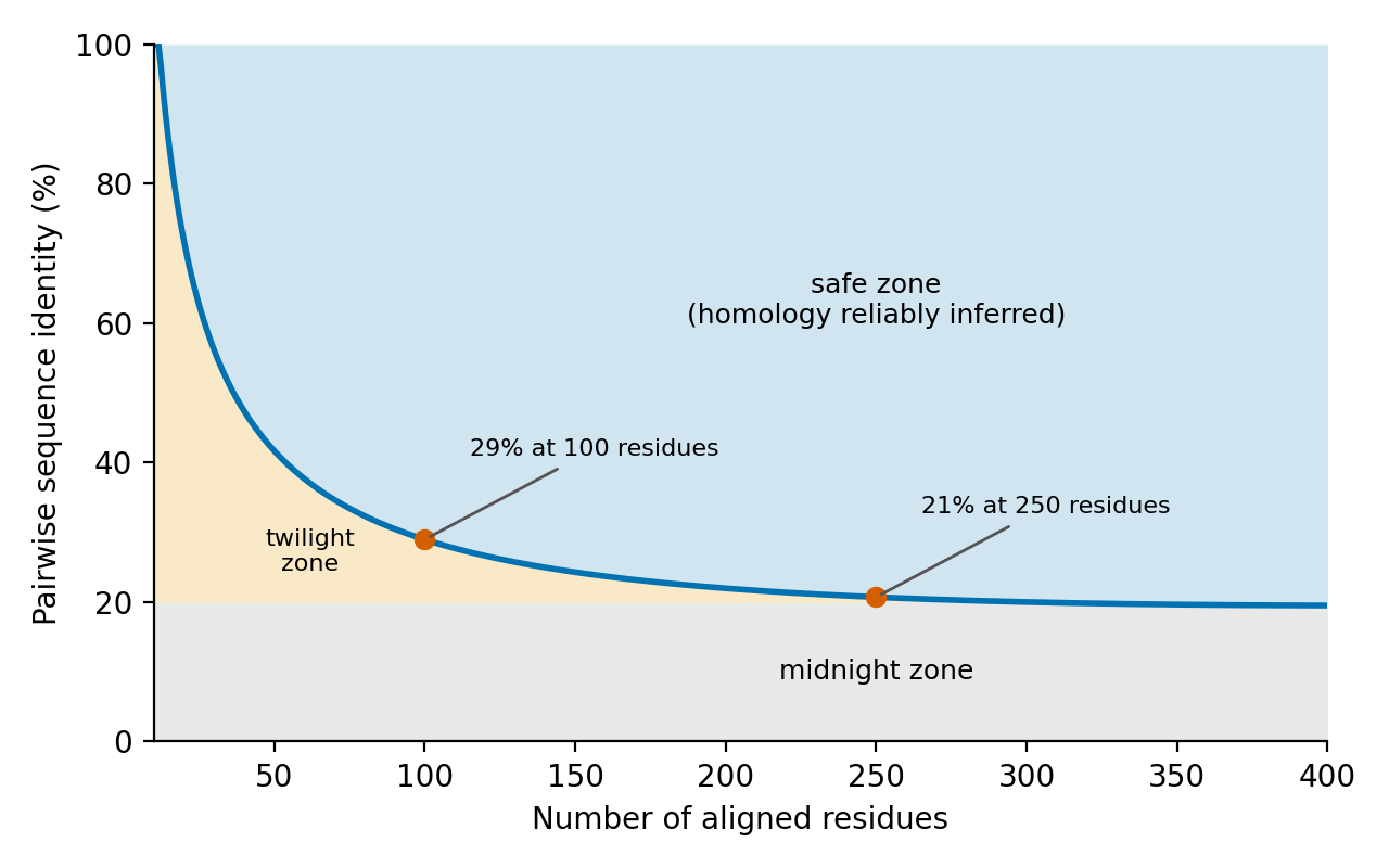
Figure 1.1: The twilight zone. The curve shows the length-dependent identity threshold of Rost (1999), \(p(L) = 480\,L^{-0.32\,(1+e^{-L/1000})}\). Above it, homology can be inferred reliably from pairwise identity. Between the curve and about 20% identity (twilight zone), true and false relationships are mixed. Below about 20% (midnight zone), identity is uninformative even though many such pairs are homologous.

Percent identity is nevertheless a poor statistic for detecting homology. It ignores the type of substitution, is sensitive to how gaps are counted, and has no direct probabilistic interpretation. Scores computed with substitution matrices and gap penalties, converted to E-values, are much better. They are the basis of every method in this chapter. Percent identity remains useful for a different purpose: describing how close two known homologues are, for example when choosing a template for homology modelling (Chapter 9) or deciding whether annotation can be transferred.

Why compare proteins rather than DNA?

When a protein-coding gene is studied, it is almost always better to compare the translated protein sequences than the DNA. There are several reasons:

  • Alphabet size. With 20 amino acids, a random match at one position occurs with a probability of about 6% (given typical amino-acid frequencies). With four nucleotides, it occurs about 25% of the time. The protein alphabet therefore carries more information per aligned position, and fewer positions are needed to reach significance.
  • Synonymous substitutions. Because of the degeneracy of the genetic code, many nucleotide changes, especially at third codon positions, do not alter the protein. They accumulate quickly and erase DNA similarity even where the protein is conserved.
  • Substitution matrices. Amino acids differ in their physicochemical properties, and the frequency with which one replaces another can be estimated from real alignments (Section 1.3). Conservative replacements can be scored as positive evidence. For DNA there is much less to exploit.
  • Composition and repeats. Genomic DNA is full of repeats and low-complexity regions that produce spurious matches.

The effect is dramatic. DNA–DNA comparisons rarely detect homology between sequences that diverged more than a few hundred million years ago, whereas protein–protein comparisons routinely detect homologues that diverged more than two billion years ago, for example between bacteria and humans (Pearson 2013). DNA comparison is the right choice for non-coding sequences (RNA genes, regulatory regions), for very closely related sequences (resequencing, read mapping; see Chapter 5), and when the reading frame is unknown. Programs such as BLASTX and TBLASTN bridge the gap by translating nucleotide sequences in all six reading frames (Section 1.4).

Structure is more conserved than sequence

The three-dimensional structure of a protein changes much more slowly than its sequence. Pairs of homologous proteins with less than 20% sequence identity often still share the same fold, with most of their core superimposable within 2–3 Å (Chothia and Lesk 1986). Below about 30% identity, however, sequence similarity no longer reliably reveals the relationship. This is why structural comparison can detect homology far beyond the limits of sequence comparison. It is also why the structural classifications SCOP, CATH and ECOD group domains into superfamilies on the basis of structural and functional evidence that sequence alone cannot provide (Murzin et al. 1995; Holm and Sander 1996; Cheng et al. 2014). With accurate predicted structures now available for almost every known protein (Jumper et al. 2021; Varadi et al. 2021), structure-based search has become a practical complement to sequence search (Section 1.4, Chapter 9). The caveat from above still applies: a shared fold is strong but not conclusive evidence of common ancestry.

Pitfalls: similarity that is not homology

The rule “significant similarity implies homology” fails in a few well-characterised situations. All of them involve sequences that violate the assumptions behind the statistics, which assume sequences composed roughly at random from standard background frequencies:

  • Low-complexity regions, such as stretches rich in a few amino acids (poly-Q, proline-rich or serine-rich segments) or short tandem repeats. These can give high scores between unrelated proteins. Search programs therefore mask them, for example with the SEG filter (Wootton and Federhen 1993), or adjust the scores for composition (Schäffer et al. 2001).
  • Biased composition and repetitive structural motifs, such as coiled coils (heptad repeats), transmembrane helices, collagen-like repeats or signal peptides. These can produce significant-looking alignments between proteins that are related only by shared physical constraints.
  • Multidomain proteins. A significant hit establishes homology only for the aligned region. Annotating a whole protein from a hit to one of its domains is a frequent source of error. So is assuming transitivity: if A is homologous to B over one domain and B to C over another, A and C need not be related at all. Before transferring an annotation, therefore, check coverage as well as significance: the fraction of the query (query coverage) and of the hit (target or subject coverage) that is included in the alignment. A highly significant hit that covers only one domain of a multidomain query supports transfer of that domain’s properties, not of the function of the whole protein. Many annotation pipelines and clustering tools (e.g. MMseqs2) require a minimum coverage of both sequences for this reason.

In addition, an E-value always refers to a particular search: one query, a database of a given size and a scoring scheme. Two different issues should be kept apart. First, the E-value of a single query already includes the size of the database (the search space): the same alignment score gives a larger E-value in a larger database. \(E = 0.01\) means that one chance hit this good is expected in a hundred such searches, whatever the database size. Second, when thousands of independent queries are searched, about \(0.01\) chance hits per query at this threshold add up over the whole experiment (ten in a thousand queries). This experiment-wide multiple-testing problem is not covered by the per-query E-value (Section 1.4).

1.2.7 Homology and the rest of this chapter

The remainder of this chapter follows from the ideas above. To measure similarity we need alignments and a scoring scheme grounded in how proteins evolve (Section 1.3). To use those scores to infer homology, we need to know their distribution for unrelated sequences, and to apply them to databases of hundreds of millions of sequences we need fast heuristics (Section 1.4). To push detection into the twilight zone we pool information from many homologues into profiles and hidden Markov models (Section 1.6). Because homology is often a property of domains rather than of whole proteins, we need domain databases (Section 1.9). The newest approach uses protein language models, trained on hundreds of millions of sequences. Their embeddings can, empirically, recover many family and structural relationships, although they are not themselves a test of common ancestry (Section 1.10).

See also: further explanation in Section D.1.1; related Wikipedia articles in Section E.1.1.

NoteSources

Parts of this section are adapted from the Wikipedia articles Homology (biology), Sequence homology, Gene, Protein and Convergent evolution (CC BY-SA 4.0, retrieved 2 October 2026).

1.3 Dynamic programming and sequence alignment

An alignment arranges two sequences in rows so that corresponding residues stand in the same column. Gaps (written -) are inserted where one sequence has gained or lost residues relative to the other. For homologous sequences, the intended interpretation is evolutionary: each column groups residues believed to derive from the same ancestral position, and the alignment is a hypothesis about the substitutions, insertions and deletions that separate the two sequences since their common ancestor (1). The algorithms themselves will align any two sequences, related or not; whether the alignment means anything biologically is a separate, statistical question. To choose between the astronomically many possible alignments we need two things:

  1. a scoring scheme, which assigns a number to each alignment so that biologically plausible alignments score higher than implausible ones; and
  2. an algorithm that finds the alignment with the best score without enumerating them all.

This section deals with both. The algorithm is dynamic programming, which finds the optimal alignment exactly, in time proportional to the product of the sequence lengths. The scoring scheme consists of a substitution matrix, which scores each pair of aligned residues, and a gap penalty, which scores insertions and deletions. Everything in this section is “exact”: given the scores, the result is guaranteed to be optimal. The heuristics that trade some of this guarantee for speed are covered in Section 1.4.

1.3.1 A short history

The mathematical idea of dynamic programming was developed by Richard Bellman at the RAND Corporation in the early 1950s, for multistage decision problems in operations research (Bellman 1954). Bellman later explained that he chose the name partly because “programming” (in the sense of planning) and “dynamic” sounded impressive and were hard to object to politically. The same principle was then discovered independently in many fields that compare sequences:

  • 1965–1966: Vladimir Levenshtein defined the edit distance between two strings, the minimum number of insertions, deletions and substitutions needed to turn one into the other.
  • 1968: Taras Vintsyuk used dynamic programming to align speech signals (the forerunner of dynamic time warping).
  • 1970: Saul Needleman and Christian Wunsch published “A general method applicable to the search for similarities in the amino acid sequence of two proteins” (Needleman and Wunsch 1970). This was the first application of dynamic programming to biological sequences and the origin of global alignment. Their original formulation scored matches only and did not penalise gaps, and as published it required time proportional to the cube of the sequence length.
  • 1972–1976: David Sankoff, Peter Sellers, Michael Waterman, Temple Smith and William Beyer put the method on a rigorous footing: Sellers showed how to compute an evolutionary distance between sequences, and Waterman, Smith and Beyer (1976) introduced general gap penalties. The same algorithm for edit distance was published in computer science by Wagner and Fischer (1974).
  • 1975: Dan Hirschberg showed how to compute the longest common subsequence in linear space, a trick later adapted to alignment.
  • 1978: Margaret Dayhoff published the PAM substitution matrices (Dayhoff et al. 1978), the first scoring scheme derived from observed evolution.
  • 1981: Temple Smith and Michael Waterman published the local alignment algorithm (Smith and Waterman 1981), in a paper of only three pages. Local alignment finds the best-matching segments of two sequences and is the basis of all database searching.
  • 1982: Osamu Gotoh showed that alignment with affine gap penalties (a cost for opening a gap plus a smaller cost for extending it) can be done in quadratic time (Gotoh 1982).
  • 1988: Eugene Myers and Webb Miller combined Gotoh’s algorithm with Hirschberg’s linear-space idea (Myers and Miller 1988).
  • 1990–1992: Samuel Karlin and Stephen Altschul derived the statistics of local alignment scores (Karlin and Altschul 1990); this also explained what substitution matrices mean. Steven and Jorja Henikoff published the BLOSUM matrices (Henikoff and Henikoff 1992), still the default for protein searches.

Since then, the algorithms themselves have changed little. The main developments have been in speed — vectorised (SIMD) and GPU implementations of Smith–Waterman, and above all the heuristics of Section 1.4 — and in scoring, where position-specific profiles (Section 1.6) replace a single substitution matrix.

1.3.2 What is dynamic programming?

Dynamic programming solves a problem by breaking it into smaller, overlapping subproblems, solving each subproblem once, storing its solution in a table and building the solution of larger problems from the stored solutions. It applies when a problem has two properties:

  • Optimal substructure (Bellman’s principle of optimality): an optimal solution to the whole problem contains optimal solutions to its subproblems.
  • Overlapping subproblems: the same subproblems recur many times, so storing their solutions (rather than recomputing them) saves time.

Sequence alignment has both properties. Consider an optimal alignment of the sequences \(A = a_1 a_2 \ldots a_n\) and \(B = b_1 b_2 \ldots b_m\). Its last column can only be one of three things: \(a_n\) aligned to \(b_m\), \(a_n\) aligned to a gap, or \(b_m\) aligned to a gap. Whichever it is, the rest of the alignment must itself be an optimal alignment of the remaining prefixes — otherwise we could replace it by a better one and improve the whole. So the best score for the prefixes \(a_1 \ldots a_i\) and \(b_1 \ldots b_j\) can be computed from the best scores of three smaller pairs of prefixes, and the problem can be solved by filling in a table of \((n+1) \times (m+1)\) prefix scores.

Why is this necessary? The number of possible alignments grows exponentially. Two sequences of length \(n\) can be aligned in \[\binom{2n}{n} \approx \frac{2^{2n}}{\sqrt{\pi n}}\] ways (counting alignments that differ only in the order of adjacent gaps in the two sequences as the same) (Durbin et al. 1998). For two proteins of 300 residues this is about \(10^{179}\) alignments, far more than could ever be enumerated. Dynamic programming finds the best one in about \(9 \times 10^4\) steps.

A useful picture is the alignment graph (or edit graph): a grid with one sequence along the top and the other down the side. Every alignment is a path from the top-left to the bottom-right corner. A diagonal step aligns two residues, a horizontal step aligns a residue of the top sequence to a gap, and a vertical step aligns a residue of the side sequence to a gap. Finding the best alignment is the same as finding the highest-scoring path through this grid — a longest-path problem in a directed acyclic graph, which is the general form of almost every dynamic programming algorithm in bioinformatics (including the Viterbi algorithm for hidden Markov models, Section 1.6).

1.3.3 Global alignment: the Needleman–Wunsch algorithm

Global alignment aligns two sequences over their entire length. It is appropriate when the sequences are expected to be homologous along their whole length, for example two orthologous proteins of similar length with the same domain structure.

Let \(s(a, b)\) be the score for aligning residue \(a\) with residue \(b\) (taken from a substitution matrix), and let each gap position cost \(d\) (a linear gap penalty; affine gaps are treated below). Define \(F(i, j)\) as the score of the best alignment of the prefixes \(a_1 \ldots a_i\) and \(b_1 \ldots b_j\). Then

\[ F(i,j) = \max \begin{cases} F(i-1, j-1) + s(a_i, b_j) & \text{align } a_i \text{ with } b_j\\[2pt] F(i-1, j) - d & a_i \text{ aligned to a gap}\\[2pt] F(i, j-1) - d & b_j \text{ aligned to a gap} \end{cases} \]

with the boundary conditions \(F(0,0) = 0\), \(F(i,0) = -i\,d\) and \(F(0,j) = -j\,d\) (a prefix aligned entirely to gaps). The table is filled row by row, so that the three cells needed for each new cell are always available. The optimal global score is \(F(n, m)\).

NEEDLEMAN-WUNSCH(A[1..n], B[1..m], s, d)
    F[0,0] ← 0
    for i ← 1 to n:  F[i,0] ← −i·d
    for j ← 1 to m:  F[0,j] ← −j·d
    for i ← 1 to n:
        for j ← 1 to m:
            F[i,j] ← max( F[i−1,j−1] + s(A[i],B[j]),    # diagonal
                          F[i−1,j]   − d,               # up: gap in B
                          F[i,j−1]   − d )              # left: gap in A
    return F[n,m]

Traceback. The table gives the optimal score; the alignment itself is recovered by tracing back from \(F(n, m)\) to \(F(0, 0)\). At each cell we ask which of the three cases produced the value (either by storing a pointer while filling the table or by recomputing the three candidates), and step to that cell. A diagonal step emits the column \(\binom{a_i}{b_j}\), a vertical step emits \(\binom{a_i}{-}\) and a horizontal step \(\binom{-}{b_j}\); the alignment is read off in reverse. When two or three cases give the same maximum, there are several co-optimal alignments with the same score. This is common, and it is a reminder that the optimal alignment is not necessarily the correct (biologically true) one.

TipWorked example: global alignment

Align GCATGCG and GATTACA with match \(+1\), mismatch \(-1\) and gap \(-1\). Each cell holds \(F(i,j)\); the blue cells and arrows show one traceback from the bottom-right corner (orange).
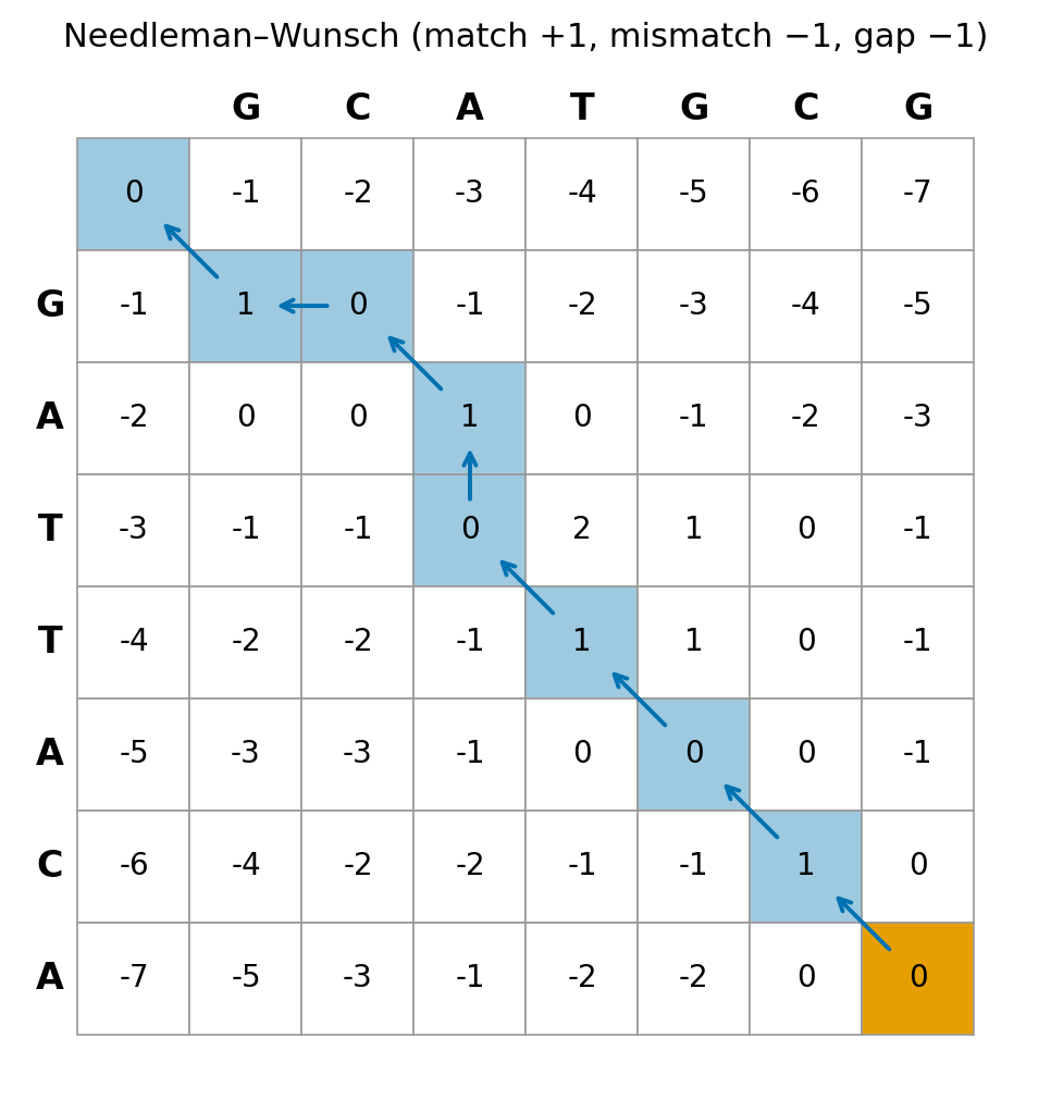
Figure 1.2: Needleman–Wunsch matrix for GCATGCG (top) and GATTACA (side), with one optimal traceback.

Needleman–Wunsch (global; match +1, mismatch −1, gap −1). Optimal score 0; there are 3 co-optimal alignments, one of which is:

GCA-TGCG
| | | | 
G-ATTACA

Check one cell: the cell for G (side) against G (top) is \(\max(0 + 1,\; -1 - 1,\; -1 - 1) = 1\), coming from the diagonal.

1.3.4 Local alignment: the Smith–Waterman algorithm

Most real problems are local. Proteins are built from domains that can be shared between otherwise unrelated proteins (Section 1.9), a query may be a fragment, and distantly related sequences may be similar only in their conserved core. A global alignment would force the dissimilar parts to be aligned too, and their noise could swamp the signal of the similar part. Local alignment instead finds the pair of segments (one from each sequence) with the highest alignment score.

Smith and Waterman’s insight was that only two changes to the global algorithm are needed (Smith and Waterman 1981):

  1. A fourth option of zero. If the best alignment ending at \((i, j)\) has a negative score, it is better to start a new alignment there:

    \[ H(i,j) = \max \begin{cases} 0 & \text{start a new local alignment}\\ H(i-1, j-1) + s(a_i, b_j)\\ H(i-1, j) - d\\ H(i, j-1) - d \end{cases} \]

    with \(H(i, 0) = H(0, j) = 0\).

  2. A different traceback. The best local alignment can end anywhere, so the traceback starts from the highest value anywhere in the matrix and stops when it reaches a cell with value zero.

Because the matrix never goes below zero, a region of poor similarity “resets” the score, and the algorithm effectively finds the best-scoring diagonal stretch, gaps included. Further, non-overlapping local alignments can be found by declumping the matrix and repeating the traceback (Waterman and Eggert, 1987), which is how programs report several alignments between the same pair of sequences.

A condition on the scoring scheme. Local alignment only makes sense if the expected score of aligning two random residues is negative: \[\sum_{a,b} p_a\, p_b\, s(a,b) < 0,\] where \(p_a\) are the background frequencies of the residues, and at least one score is positive. If the expected score were positive, any long random alignment would accumulate a positive score, and the “local” alignment would simply extend over the full length of both sequences — the algorithm would behave like global alignment. All standard substitution matrices satisfy this condition, for a reason explained under Substitution matrices below.

TipWorked example: local alignment

Align TGTTACGG and GGTTGACTA with match \(+3\), mismatch \(-3\) and a linear gap penalty of \(2\) per position. Negative values never appear; the traceback starts at the maximum (13, orange) and stops at the first zero.
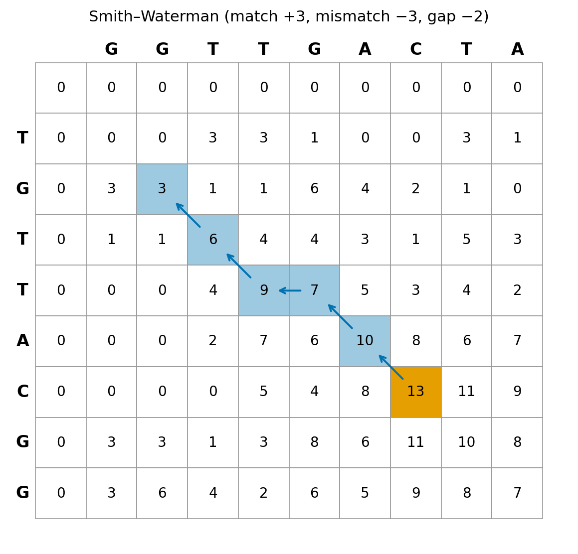
Figure 1.3: Smith–Waterman matrix for TGTTACGG (side) and GGTTGACTA (top). The best local alignment contains one gap.

Smith–Waterman (local; match +3, mismatch −3, gap −2). Highest cell 13; the traceback stops at the first zero and gives the local alignment:

GTT-AC
||| ||
GTTGAC

The alignment score is \(5 \times 3 - 2 = 13\): five matches and one gap position.

1.3.5 Other alignment modes

Between fully global and fully local there are useful intermediate forms, all obtained by changing the boundary conditions and the cells where the traceback starts and stops:

  • Semi-global (“glocal” or end-gap-free) alignment aligns all of one sequence to part of another — for example a short read to a genome, or a domain to a full-length protein. Leading and trailing gaps in the longer sequence are not penalised: the first row is initialised to zero, and the traceback starts from the best cell in the last row.
  • Overlap alignment allows free end gaps in both sequences, so that the end of one sequence is aligned to the start of the other. It is used to detect overlaps between reads in genome assembly (Chapter 5).
  • Banded alignment restricts the computation to a band of width \(k\) around a diagonal. This reduces the cost to \(O(k\,n)\) and is exact if the optimal path is known to stay within the band, as when two sequences are already known to be very similar. Banded dynamic programming is used to refine the hits of heuristic methods (Section 1.4).

1.3.6 Edit distance: maximising similarity or minimising distance

Alignment can be framed in two equivalent ways. Similarity scores are maximised: matches score positively and mismatches and gaps negatively, as above. Distances are minimised: each operation has a non-negative cost. The simplest distance is the Levenshtein or edit distance, the minimum number of single-character substitutions, insertions and deletions needed to transform one string into the other. It is computed by the same recursion with \(\min\) instead of \(\max\), a cost of 1 for each mismatch or gap and 0 for a match. For global alignment with suitable parameters, the two formulations give the same optimal alignments. Local alignment, however, has no natural distance formulation — a distance can always be made smaller by aligning shorter segments — which is one reason why bioinformatics works with similarity scores.

1.3.7 Gap penalties

Insertions and deletions (indels) arise from replication slippage, unequal crossing-over, transposition and other events, and one event often inserts or deletes several residues at once. A good gap penalty should therefore make one gap of length 3 cheaper than three separate gaps of length 1. Several forms are used; let \(w(k)\) be the penalty for a gap of length \(k\):

Gap penalty \(w(k)\) Comment
Linear \(k\,d\) Simplest; every gap position costs the same, so long gaps are over-penalised and gaps tend to be scattered.
Constant \(g\) Gap length does not matter; sometimes used for genomic DNA.
Affine \(g_o + (k-1)\,g_e\) with \(g_o > g_e\) A cost for opening a gap plus a smaller cost for each extension. The standard choice.
Convex (e.g. logarithmic) \(g_o + g_e \log k\) Each additional gap position costs less than the previous one; fits observed indel length distributions better, but is more expensive to compute.
General any function Needs \(O(n^2 m)\) time, as in the original Smith–Waterman paper.

(Some programs, such as BLAST, define the affine penalty as \(g_o + k\,g_e\), counting the extension cost for every position including the first; the parameters are then not directly comparable between programs.) Typical affine parameters for proteins are an opening penalty of about 10–12 and an extension penalty of 0.5–2 in units of the substitution matrix; BLAST with BLOSUM62 uses 11 and 1 by default.

The difference matters in practice. With a linear gap penalty the alignments of TACGGGCCCGCTAC and TAGCCCTATCGGTCA contain several isolated gap positions; with an affine penalty the same sequences align with a few longer gaps — fewer, biologically more plausible, indel events.

Affine gaps in quadratic time: Gotoh’s algorithm

With a general gap function, each cell must consider gaps of every possible length ending there, which gives \(O(n^2 m)\) time. Gotoh showed that for affine penalties it is enough to keep three matrices, one for each possible state of the last column (Gotoh 1982):

  • \(M(i,j)\): best score of an alignment of the prefixes that ends with \(a_i\) aligned to \(b_j\);
  • \(I_x(i,j)\): best score of an alignment that ends with \(a_i\) aligned to a gap (a gap in \(B\));
  • \(I_y(i,j)\): best score of an alignment that ends with \(b_j\) aligned to a gap (a gap in \(A\)).

With an affine penalty \(w(k) = g_o + (k-1) g_e\) the recursions are

\[ \begin{aligned} M(i,j) &= s(a_i, b_j) + \max\{M(i-1,j-1),\; I_x(i-1,j-1),\; I_y(i-1,j-1)\}\\ I_x(i,j) &= \max\{M(i-1,j) - g_o,\;\; I_x(i-1,j) - g_e\}\\ I_y(i,j) &= \max\{M(i,j-1) - g_o,\;\; I_y(i,j-1) - g_e\} \end{aligned} \]

and the score of the best alignment is the maximum of the three matrices in the final cell. (This version forbids a gap in \(A\) to be directly followed by a gap in \(B\), which is never optimal when \(s\) is not too negative.) Opening a gap means leaving the match state; extending it means staying in the gap state. Each cell is still computed in constant time, so the cost remains \(O(nm)\). The local version adds the zero option to \(M\). Gotoh’s original traceback procedure contained an error that could miss the optimal alignment in some cases; this was pointed out and corrected by Altschul and Erickson (1986).

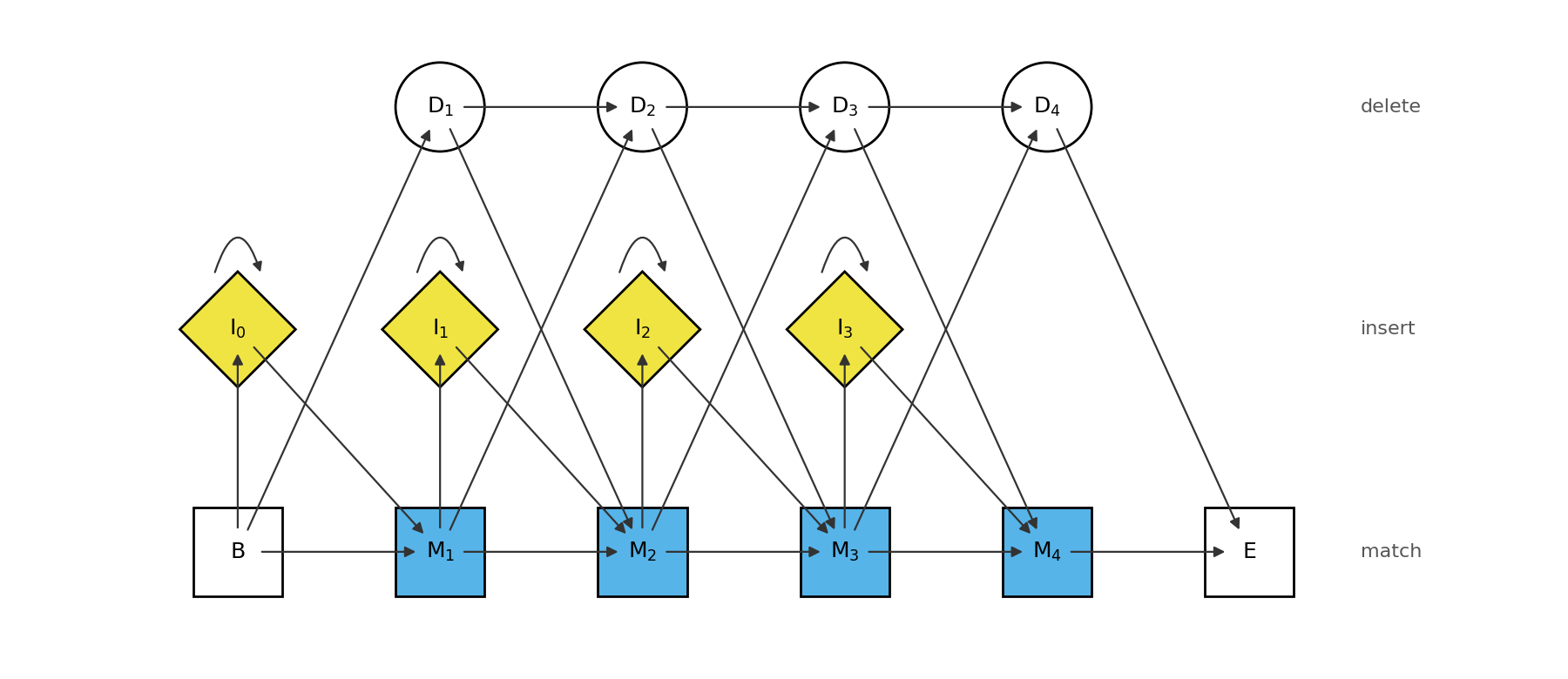
The three matrices can be seen as the three states of a small finite-state machine — match, insertion, deletion — with transitions whose costs are the gap-opening and gap-extension penalties. This is exactly the structure of a pair hidden Markov model, in which the scores become log-probabilities (Durbin et al. 1998). Profile HMMs (Section 1.6) extend the same idea to whole families of sequences.

1.3.8 Time and space complexity

Filling one cell takes constant time, so all variants above need \(O(nm)\) time. Storing the full matrix for the traceback needs \(O(nm)\) space. For two proteins this is trivial, but for two sequences of 100,000 residues it already amounts to \(10^{10}\) cells.

Linear space. The score alone needs only the previous row, so it can be computed in \(O(\min(n, m))\) space. To recover the alignment in linear space, Hirschberg’s divide-and-conquer method is used:

  1. Compute the scores of the forward alignments of the top half of \(A\) against all prefixes of \(B\), and the scores of the reverse alignments of the bottom half of \(A\) against all suffixes of \(B\), keeping only the last row of each.
  2. The optimal path must cross the middle row of \(A\) at the column \(j\) where the sum of the forward and reverse scores is maximal. This splits the problem into two independent subproblems — top-left and bottom-right of that point.
  3. Recurse on each half.

The total work is about twice that of the ordinary algorithm, still \(O(nm)\), while the space is \(O(n + m)\). Myers and Miller extended this to affine gap penalties (Myers and Miller 1988), and it is the basis of space-efficient alignment tools.

Faster than quadratic? The “Four Russians” technique reduces the time to \(O(nm / \log n)\) for small alphabets, but has little practical importance. More importantly, there is strong theoretical evidence that edit distance cannot be computed in strongly subquadratic time in the worst case. In practice, Smith–Waterman is accelerated by computing many cells at once: SIMD instructions on ordinary processors (as in the SSEARCH program of the FASTA package and in the SWIPE and Parasail libraries) and GPUs reach billions of cell updates per second.

Even so, exact local alignment of every query against a large database is expensive. UniProt contains roughly \(10^{11}\) residues, so comparing one 300-residue protein against all of it requires about \(3 \times 10^{13}\) cell updates — minutes to hours on a modern computer, for a single query. Comparing all proteins of a newly sequenced genome, or a metagenome with millions of proteins, against the database would take years. This is the motivation for the heuristic methods of Section 1.4.

1.3.9 Substitution matrices

The algorithm guarantees the optimal alignment for a given scoring scheme; whether that alignment is biologically meaningful depends entirely on the scores. For DNA, simple schemes are often adequate. For proteins, the 20 amino acids differ greatly in size, charge, polarity and other properties, and some substitutions (for example isoleucine to valine) are accepted by evolution far more often than others (for example tryptophan to glycine). A substitution matrix is a \(20 \times 20\) table of scores \(s(a, b)\) that captures these differences.

Scores as log-odds ratios

Substitution scores are best understood as log-odds scores comparing two hypotheses about an aligned pair of residues \(a\) and \(b\):

  • the match (homology) model, in which \(a\) and \(b\) are derived from a common ancestral residue and occur together with target frequency \(q_{ab}\), estimated from alignments of true homologues; and
  • the random model, in which \(a\) and \(b\) are unrelated and occur together with probability \(p_a p_b\), the product of their background frequencies.

The score is the logarithm of the ratio of these probabilities,

\[ s(a,b) = \frac{1}{\lambda} \log \frac{q_{ab}}{p_a\, p_b}, \]

where \(\lambda\) is a scale factor chosen so that the scores can be rounded to convenient integers. Matrices are usually given in bits (logarithm base 2) or fractions of bits; BLOSUM62, for example, is in half-bit units, so a score of \(+2\) means the pair is \(2^{2/2} = 2\) times more likely under the homology model than by chance. A positive score means the pair occurs more often in true alignments than expected by chance, a negative score that it occurs less often, and zero that there is no information.

Because scores are logarithms of probability ratios, and positions in an ungapped alignment are treated as independent, the total score of an ungapped alignment is the log-likelihood ratio of the whole alignment: \[S = \sum_{k} s(x_k, y_k) = \frac{1}{\lambda} \log \frac{P(\text{alignment} \mid \text{homologous})}{P(\text{alignment} \mid \text{random})}.\] Dynamic programming thus finds the alignment that is most likely under the homology model relative to the random model. The same interpretation underlies profile scores and hidden Markov models (Section 1.6).

Two further consequences follow:

  • The expected score is always negative. The expected score of a random pair is \[\sum_{a,b} p_a p_b\, s(a,b) = -\frac{1}{\lambda} \sum_{a,b} p_a p_b \log \frac{p_a p_b}{q_{ab}} \le 0,\] because the sum on the right is a relative entropy (Kullback–Leibler divergence), which is never negative. Any log-odds matrix therefore automatically satisfies the requirement of local alignment.
  • Every matrix is a log-odds matrix. Karlin and Altschul showed the converse (Karlin and Altschul 1990): for any scoring matrix with a negative expected score and at least one positive entry, there is a unique \(\lambda > 0\) with \(\sum_{a,b} p_a p_b\, e^{\lambda s(a,b)} = 1\), and \(q_{ab} = p_a p_b\, e^{\lambda s(a,b)}\) are the target frequencies for which the matrix is optimal. Choosing a matrix is therefore always, implicitly, choosing what kind of alignments one expects to find. The same \(\lambda\) appears in the statistics of alignment scores (Section 1.4).

The relative entropy \[H = \sum_{a,b} q_{ab} \log_2 \frac{q_{ab}}{p_a p_b}\] is the average score per aligned position in true alignments, in bits. It measures how much information each aligned pair carries for distinguishing homology from chance (Altschul 1991). Matrices for closely related sequences have high relative entropy (each position is informative, so a short alignment suffices); matrices for distant relationships have low relative entropy (a longer alignment is needed to reach significance).

Scoring DNA

For nucleotides, a simple match/mismatch scheme is usually used, for example \(+1/-2\) or \(+2/-3\) for highly similar sequences and \(+1/-1\) for more divergent ones (the ratio sets the implied target identity). Since transitions (purine–purine or pyrimidine–pyrimidine changes, A↔︎G and C↔︎T) are about twice as common as transversions in most genomes, they can be given a less negative score. For protein-coding genes, alignment of the translated sequences is far more sensitive than DNA alignment, because the genetic code is degenerate and synonymous changes saturate quickly.

PAM matrices

The first substitution matrices derived from evolutionary data were Margaret Dayhoff’s PAM matrices (Dayhoff et al. 1978). A point accepted mutation is the replacement of one amino acid by another that has been accepted by natural selection, that is, has become fixed in the population. Dayhoff’s approach was explicitly evolutionary:

  1. Data. 1572 accepted substitutions were counted on the branches of phylogenetic trees reconstructed for 71 families of closely related proteins (at least 85% identical), so that each observed difference could be assumed to be a single substitution.
  2. Mutation probability matrix. From the counts, together with the mutability of each amino acid (how often it changes relative to how often it occurs) and the amino-acid frequencies, a matrix \(M_1\) of transition probabilities was computed, scaled so that on average 1% of the amino acids change. This is PAM1: one accepted point mutation per 100 residues.
  3. Extrapolation. Evolution was modelled as a Markov chain, so the matrix for a longer evolutionary distance is a power of \(M_1\): \(M_n = M_1^{\,n}\). PAM250 corresponds to 250 accepted mutations per 100 residues — many positions have changed several times — and to about 20% sequence identity.
  4. Log-odds scores. The PAM\(n\) score is \(s(i,j) = 10 \log_{10} \bigl(M_n(i,j) / f_i\bigr)\), the probability that \(j\) has become \(i\) after \(n\) PAM units relative to the background frequency of \(i\).

Dayhoff found that asparagine, serine and aspartate are among the most mutable amino acids, and cysteine and tryptophan the least, in line with their special structural roles. The main weakness of PAM is the extrapolation: the substitution pattern of very similar sequences, which is dominated by single-nucleotide changes in the codon, is assumed to hold over long distances. The data set was also small by modern standards. Later matrices of the same type, such as JTT (1992) and WAG (2001), were estimated from much larger data sets and are used as substitution models in phylogenetics (Chapter 4).

BLOSUM matrices

Steven and Jorja Henikoff took a different, empirical approach (Henikoff and Henikoff 1992). Instead of extrapolating from close relatives, they counted substitutions directly in conserved regions of distantly related proteins:

  1. Data. The BLOCKS database contains ungapped multiple alignments (“blocks”) of the most conserved regions of protein families — about 2000 blocks from more than 500 families in the original work.
  2. Clustering. To avoid over-counting closely related sequences, the sequences in each block that are more than \(r\)% identical are clustered, and each cluster contributes with a total weight of one sequence.
  3. Counting. All pairs of amino acids in each column, between sequences in different clusters, are counted. This gives the observed pair frequencies \(q_{ab}\), and from them the background frequencies \(p_a\).
  4. Log-odds scores. \(s(a,b) = 2 \log_2 \bigl(q_{ab} / (p_a p_b)\bigr)\), rounded to the nearest integer (half-bit units).

The number in the name is the clustering threshold: BLOSUM62 is computed from blocks in which sequences more than 62% identical were clustered together. A higher number means less clustering, more similar sequences contribute and the matrix is suited to closely related sequences; a lower number suits distant relationships. The numbering therefore runs in the opposite direction to PAM. For PAM, a higher number means a greater evolutionary distance (more accepted mutations); for BLOSUM, a lower number is intended for more divergent sequences. BLOSUM80 corresponds roughly to a low PAM number, BLOSUM45 to a high one. The two numbers measure different things (an extrapolated distance and a clustering threshold) and cannot be compared directly.

In comparisons with PAM, BLOSUM matrices performed better in database searches, especially for distant relationships, and BLOSUM62 became the default of BLAST and most other protein search programs. Its relative entropy is about 0.70 bits per position, similar to PAM160; BLOSUM45 (about 0.38 bits) is comparable to PAM250. The derivation of BLOSUM62, and why it works so well, is explained in a short and very readable note by Eddy (2004b). A curious footnote is that the program originally used to compute BLOSUM62 contained errors, discovered only in 2008. The “correct” matrix turned out to perform slightly worse in searches than the miscalculated one, which is still the standard — a reminder that the best matrix is ultimately an empirical question.

Choosing a matrix

Because each matrix is optimal for a particular evolutionary distance — its implicit target frequencies — the best matrix depends on what one is looking for (Altschul 1991):

Purpose Typical matrices
Very similar sequences, short queries or short peptides PAM30, PAM70, BLOSUM80
General database searching BLOSUM62 (the usual default)
Distant relationships, long alignments BLOSUM45, PAM250

A “deep” matrix (low relative entropy) can detect distant homologues but needs long alignments to give significant scores, and it tends to extend alignments into unrelated regions. A “shallow” matrix (high relative entropy) gives short, accurate alignments of close relatives but misses distant ones. Some programs therefore search with several matrices, and modern programs adjust the matrix to the amino-acid composition of the sequences being compared (composition-based statistics), which matters for proteins with unusual compositions such as transmembrane or low-complexity proteins.

Limitations of a single substitution matrix

A substitution matrix assumes that the same substitution pattern applies at every position of every protein. In reality, a buried hydrophobic position, a catalytic residue and a surface loop evolve very differently. Position-specific scores, estimated from a multiple alignment of the family, capture this variation and are the basis of profiles and profile HMMs (Section 1.6); environment-specific matrices, which depend on the structural context of each residue, are used in fold recognition (Chapter 9).

1.3.10 From scores to significance

An optimal alignment always exists, even between two random sequences. The scores of optimal local alignments between unrelated sequences are not normally distributed but follow an extreme-value (Gumbel) distribution, because each score is itself the maximum over many possible alignments. Karlin and Altschul derived its parameters for ungapped alignments (Karlin and Altschul 1990): the expected number of alignments with score at least \(S\) between random sequences of lengths \(m\) and \(n\) is

\[E = K\, m\, n\, e^{-\lambda S},\]

with \(\lambda\) the same scale factor as above and \(K\) a second constant that depends on the scoring system. For gapped alignments the parameters are estimated by simulation. These E-values, and their use in database searches, are treated in Section 1.4. Global alignment scores have no comparably simple theory, and their significance is usually assessed by shuffling the sequences.

1.3.11 Summary

  • Dynamic programming finds the optimal alignment of two sequences under a given scoring scheme exactly, in \(O(nm)\) time, by building optimal alignments of prefixes from optimal alignments of shorter prefixes.
  • Global (Needleman–Wunsch), local (Smith–Waterman), semi-global and overlap alignment differ only in their boundary conditions, the zero option and where the traceback starts and stops.
  • Affine gap penalties are handled in quadratic time with three matrices (Gotoh), and alignments can be recovered in linear space (Hirschberg, Myers–Miller).
  • Substitution scores are log-odds ratios of target and background frequencies. Every matrix implies a set of target frequencies and is best suited to one evolutionary distance; PAM extrapolates from close relatives, BLOSUM counts directly in conserved blocks.
  • The optimal alignment is only as good as the scoring scheme, and an optimal alignment is not necessarily the true one. Whether a score indicates homology is a statistical question (Section 1.4), and for sequence identities below about 25–30% the answer is often uncertain (1).

See also: further explanation in Section D.1.2; related Wikipedia articles in Section E.1.2.

NoteSources

Parts of this section are adapted from the Wikipedia articles Dynamic programming, Sequence alignment, Needleman–Wunsch algorithm, Smith–Waterman algorithm, Hirschberg’s algorithm, Gap penalty, Substitution matrix, BLOSUM and Point accepted mutation (CC BY-SA 4.0, retrieved 2 October 2026). The worked examples follow those in the Needleman–Wunsch and Smith–Waterman articles.

1.4 Heuristic search methods

Dynamic programming (Section 1.3) is guaranteed to find the best alignment for a given scoring scheme, but it is expensive. Comparing a query of length \(m\) with a database of total length \(N\) takes time proportional to \(mN\). For a typical protein of 300 residues searched against UniProtKB, with a few hundred million sequences, that means tens of trillions of dynamic-programming cells for every query. Even with modern vectorised implementations, which can fill billions of cells per second, this takes hours. Databases have also grown much faster than computers have become faster: sequence databases have roughly doubled every two years since the 1980s, and metagenomic projects now produce billions of protein sequences.

Practical database searching therefore uses heuristics: methods that first find short, promising regions of similarity quickly, and then spend the expensive dynamic-programming effort only on those regions. The price is that a heuristic can miss alignments that the full Smith–Waterman algorithm would have found. The heuristic lies mainly in the filter, the decision which sequences and regions are examined at all. The alignments that are finally reported are computed by dynamic programming, usually restricted to a band or by X-drop extension around the seed. For clear homologues they are therefore usually identical, or very close, to the Smith–Waterman alignment, although an X-drop extension can stop early and report a shorter alignment. The art of designing a search tool lies in choosing a filter that discards almost all unrelated sequences while keeping almost all true homologues. Equally important is the second half of the problem: deciding which of the reported hits are significant. This section covers both, from FASTA and BLAST to the tools used today for searching billions of sequences and structures, and the exact-matching indexes used for mapping sequencing reads.

1.4.1 FASTA

The first widely used heuristic was developed by David Lipman and William Pearson. FASTP, for protein searches, was published in 1985 (Lipman and Pearson 1985). Its successor FASTA, which extended the approach to nucleotide and translated protein–DNA searches, followed in 1988 (Pearson and Lipman 1988). The name lives on in the FASTA file format, which was introduced with the program and is now the standard way to store sequences.

FASTA builds on a simple observation. If two sequences are related, their alignment usually contains several short stretches of identical residues, and these lie on the same diagonal of the dot plot (the same offset between the two sequences). FASTA proceeds in four steps:

  1. Find word hits. All identical words of length ktup (typically 1 or 2 for proteins, 4–6 for DNA) shared by the query and the database sequence are found with a lookup table. The time needed is proportional to the sequence lengths, not to their product.
  2. Find the best diagonal regions. Hits on the same diagonal are grouped, and each diagonal region is scored by the number of hits minus a penalty for the distance between them. The ten best regions are kept and rescored with a substitution matrix (originally PAM250, now BLOSUM50 by default), which allows conservative substitutions and runs of identities shorter than ktup to contribute. The best single region gives the score init1.
  3. Join regions. Regions on nearby diagonals are combined into one longer alignment containing gaps, at a cost of a joining penalty. The score of the best combination is initn.
  4. Optimise. For the best-scoring database sequences, a banded Smith–Waterman alignment is computed in a narrow band (for example 32 residues wide) around the best diagonal. This gives the final score opt.

A smaller ktup makes the search more sensitive but slower. A distinctive feature of FASTA is how it estimates significance. Because a database search compares the query with many sequences, most of which are unrelated, the distribution of their scores can itself serve as the null model. FASTA fits an extreme-value distribution to the scores of the unrelated sequences and reports an expectation value for each hit (Pearson 2013). The FASTA package also contains SSEARCH, a full Smith–Waterman implementation that is often used as a gold standard for sensitivity.

1.4.2 BLAST

The Basic Local Alignment Search Tool was published in 1990 by Stephen Altschul, Warren Gish, Webb Miller, Eugene Myers and David Lipman at the NCBI (Altschul et al. 1990). It became one of the most cited papers in all of science. BLAST combined two ideas. The first was a faster and more selective seeding strategy than FASTA’s. The second, at least as important, was a rigorous statistical theory for local alignment scores, developed in parallel by Samuel Karlin and Altschul (Karlin and Altschul 1990) and described below.

The original algorithm (1990)

BLAST looks for high-scoring segment pairs (HSPs): pairs of equal-length segments, one from each sequence, aligned without gaps, whose score cannot be improved by extending or shortening them. The highest-scoring of these is the maximal segment pair (MSP). The original BLAST approximated the MSP score in three steps.

  1. Compile a word list. The query is split into all overlapping words of length \(w\) (usually \(w = 3\) for proteins). For each query word, BLAST lists all words of the same length that score at least \(T\) against it with the substitution matrix (BLOSUM62 by default). These are the neighbourhood words. For example, with BLOSUM62 the query word PQG scores 15 against PEG (\(7 + 2 + 6\)) and 12 against PQA (\(7 + 5 + 0\)). With \(T = 13\), PEG is in the neighbourhood of PQG but PQA is not. The neighbourhood is what distinguishes BLAST from FASTA: seeds do not have to be identical, only similar, so they are much more informative. For DNA, BLAST instead uses exact matches of a longer word (by default \(w = 11\)).
  2. Scan the database. The neighbourhood words are compiled into a finite-state automaton (or a lookup table), so that each database sequence can be scanned in a single pass for exact occurrences of any of them. Each occurrence is a hit.
  3. Extend the hits. Each hit is extended in both directions without gaps, adding the substitution scores residue by residue. The extension stops when the running score has fallen more than \(X\) below the best score seen so far (the X-drop rule). The best segment found is reported as an HSP if its score is high enough.

The parameter \(T\) controls the trade-off between speed and sensitivity. A high \(T\) gives few neighbourhood words and few hits to extend, so the search is fast but may miss alignments that contain no high-scoring word. A low \(T\) gives the opposite.

Gapped BLAST and the two-hit method (1997)

The 1990 BLAST reported only ungapped alignments. A real alignment interrupted by indels therefore appeared as several separate HSPs, and weak alignments could be missed altogether. In 1997, Altschul and co-workers published gapped BLAST together with PSI-BLAST (Altschul et al. 1997), with two main improvements.

  • The two-hit method. Most time in the original BLAST was spent extending hits that led nowhere. The authors observed that a biologically meaningful HSP is usually much longer than a single word, so it will typically contain two word hits on the same diagonal. In gapped BLAST, an ungapped extension is triggered only when two non-overlapping hits occur on the same diagonal within a distance \(A\) (by default 40 residues) of each other. This allowed \(T\) to be lowered, increasing sensitivity, while the number of extensions fell sharply.
  • Gapped extension. If an ungapped HSP scores above a moderate threshold, a gapped alignment is computed by dynamic programming, starting from a central residue pair of the HSP and extending in both directions. The extension uses the X-drop rule: cells whose score has fallen more than \(X_g\) below the best score are not explored. This confines the computation to a small region around the seed rather than the whole matrix.

The result was a program about three times faster than the original, which reports gapped alignments. PSI-BLAST, the iterative profile search introduced in the same paper, is described in Section 1.6.

Low-complexity filtering

Regions of biased composition, such as stretches rich in a single amino acid, short tandem repeats or coiled coils, align with high scores to many unrelated sequences. Because they violate the assumptions of the statistical model, they produce many false positives with apparently excellent E-values. Such hits can be very strong and still biologically meaningless: two proteins that both contain a polyglutamine or a proline-rich stretch are not thereby homologous. Two remedies are used. Masking identifies low-complexity regions in the query, with SEG (Wootton and Federhen 1993) for proteins and DUST for DNA, and replaces them by X (protein) or N (DNA) so that they cannot seed alignments (soft masking excludes them from seeding only, but allows them in the extension). Composition-based statistics (Schäffer et al. 2001) instead adjust the scores of each alignment to the amino-acid composition of the two sequences (see below). Which of these is on by default differs between programs and versions (in current BLAST+, DUST masking is the default for blastn, and composition-based statistics rather than SEG for blastp), so the settings should be checked and reported. Masking is also a common reason why a search misses a hit that seems obvious.

The BLAST family of programs

The same engine is used in a family of programs that differ in what is compared with what:

Program Query Database Typical use
blastp protein protein find homologues of a protein
blastn nucleotide nucleotide DNA/RNA similarity
megablast nucleotide nucleotide very similar sequences (long exact seeds, \(w = 28\)); fast
blastx nucleotide, translated in six frames protein find what protein a DNA fragment or transcript encodes
tblastn protein nucleotide, translated in six frames find (unannotated) genes for a protein in genomes
tblastx translated nucleotide translated nucleotide compare two DNA sequences at the protein level; slow

Translated searches are important because protein sequences diverge much more slowly than the DNA that encodes them. Two genes whose DNA is no longer recognisably similar, because of synonymous changes and codon usage, may still encode clearly similar proteins. In general, searching at the protein level is far more sensitive than at the DNA level. Translated searches are also how nucleotide data (genomes, transcripts, metagenomic reads) are connected to the protein databases, where most functional annotation lives. Two practical points follow from the translation. The search space is measured in amino-acid residues, so a translated nucleotide sequence contributes about a third of its length per reading frame. And a sequencing error that causes a frameshift splits a translated alignment into pieces in different frames; some tools, such as FASTX and FASTY in the FASTA package and DIAMOND’s frameshift-aware mode, can align across such frameshifts.

BLAT and other genome-scale tools

BLAST builds its word index from the query and scans the database. For aligning millions of mRNAs or ESTs to a genome, the reverse is more efficient. BLAT, the BLAST-like alignment tool written by Jim Kent for the human genome project (Kent 2002), builds an index of non-overlapping \(k\)-mers of the whole genome, keeps it in memory, and then looks up the \(k\)-mers of each query. It is designed for finding very similar sequences (for example the same gene in the same or a closely related species) and is hundreds of times faster than BLAST for that task, but much less sensitive for distant homologues. The same idea, an index of the reference, underlies the read mappers discussed at the end of this section. Aligning whole genomes to each other, where rearrangements, duplications and repeats must be handled, needs further steps, described in Section 1.8.

1.4.3 The statistics of alignment scores

Every search reports a best hit, even for a random query. The crucial question is therefore not “how similar is the hit?” but “how often would we see a score this high by chance?” Answering it requires knowing the distribution of scores between unrelated sequences.

Why not a normal distribution?

The score of an alignment of two fixed segments is a sum of many substitution scores, and so by the central limit theorem it is approximately normally distributed. But a local alignment score is the maximum over all possible pairs of segments. The maximum of many random variables does not follow a normal distribution. Its distribution belongs to the family of extreme value distributions, and for local alignment scores it is of the Gumbel type. The Gumbel distribution has a much heavier right tail than a normal distribution: it decays exponentially, as \(e^{-\lambda x}\), whereas the normal tail falls off as \(e^{-x^2/2}\). Using a normal model, or a z-score, therefore greatly underestimates how often high scores occur by chance.
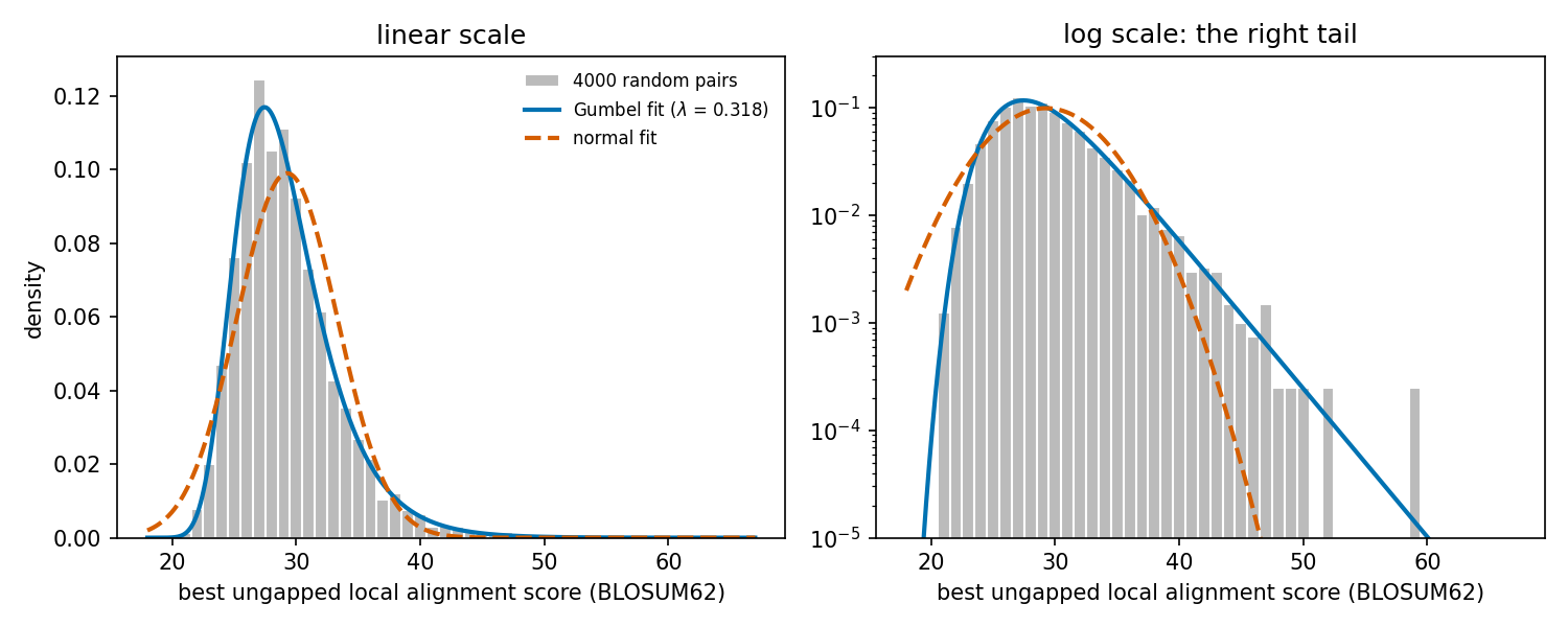
Figure 1.4: Distribution of the best ungapped local alignment score between pairs of random protein sequences (length 250, BLOSUM62). A Gumbel distribution (blue) fits the data, including the right tail; a normal distribution fitted to the same data (orange, dashed) underestimates the probability of high scores by orders of magnitude.

In this simulation (4000 pairs of random sequences of length 250, BLOSUM62, background frequencies of Robinson & Robinson), the fitted Gumbel distribution has \(\lambda \approx 0.318\) and \(K \approx 0.099\), close to the value \(\lambda = 0.318\) predicted by solving \(\sum_{ij} p_i p_j e^{\lambda s_{ij}} = 1\). For a score of 48, the Gumbel model gives \(P(S \ge x) = 1.5 \times 10^{-3}\), whereas a normal distribution fitted to the same data gives \(1.7 \times 10^{-6}\): the normal model underestimates how often high scores occur by chance.

Karlin–Altschul statistics

For ungapped local alignments, Karlin and Altschul derived the score distribution analytically (Karlin and Altschul 1990). The theory assumes:

  • the residues of the two sequences are independent and drawn from background frequencies \(p_i\);
  • the expected score of aligning two random residues is negative, \(\sum_{ij} p_i p_j s_{ij} < 0\) (otherwise the best “local” alignment would grow with the length of the sequences and become a global one);
  • at least one score \(s_{ij}\) is positive.

Under these conditions, for two random sequences of lengths \(m\) and \(n\) that are long enough, the number of distinct HSPs with score at least \(S\) is approximately Poisson-distributed with mean

\[ E = K\,m\,n\,e^{-\lambda S}. \]

This is the E-value: the number of alignments with score \(\ge S\) expected by chance. Two parameters depend on the scoring system and the background frequencies. \(\lambda\) is the unique positive solution of

\[ \sum_{i,j} p_i\, p_j\, e^{\lambda s_{ij}} = 1, \]

and acts as a scale that converts raw scores into natural units. \(K\) is a smaller correction factor for the fact that high-scoring alignments are not independent: an HSP is usually surrounded by overlapping, slightly lower-scoring ones. For BLOSUM62 with standard amino-acid frequencies, \(\lambda \approx 0.318\) and \(K \approx 0.13\) for ungapped alignments. Equivalently, the maximal score follows a Gumbel distribution,

\[ P(S \ge x) \approx 1 - \exp\!\left(-e^{-\lambda (x - \mu)}\right), \qquad \mu = \frac{\ln (K m n)}{\lambda}. \]

The theory also connects to substitution matrices (Section 1.3). Every scoring matrix with negative expected score is implicitly a log-odds matrix, \(s_{ij} = \frac{1}{\lambda} \ln \frac{q_{ij}}{p_i p_j}\), for some target frequencies \(q_{ij}\). These are the frequencies with which residue pairs occur in the alignments the matrix is best at finding.

E-values, P-values and bit scores

Raw scores depend on the scoring system, so they cannot be compared between searches that use different matrices. Normalising with \(\lambda\) and \(K\) gives the bit score

\[ S' = \frac{\lambda S - \ln K}{\ln 2}, \]

in terms of which the E-value takes a particularly simple form:

\[ E = m\,n\,2^{-S'}. \]

Every extra bit of score halves the E-value. The “search space” \(mn\) appears explicitly: in a database search, \(n\) is the total length of the database. Since the number of chance HSPs is Poisson-distributed, the probability of finding at least one with score \(\ge S\) is the P-value

\[ P = 1 - e^{-E}. \]

For small values, \(P \approx E\). For large values they differ: \(E = 3\) means that about three such hits are expected by chance, but \(P\) can never exceed 1. BLAST therefore reports E-values, which are easier to interpret over the whole range.

Corrections and gapped alignments

Several refinements are needed in practice.

  • Edge effects. An alignment cannot start near the end of a sequence and still be long. BLAST therefore uses effective lengths: \(m\) and \(n\) are shortened by the expected length of an HSP, \(\ell \approx \ln(Kmn)/H\), where \(H\) is the relative entropy of the scoring system. For a database of many sequences, the correction is applied to each sequence.
  • Gapped alignments. No exact theory exists for gapped alignments. Simulations show that their scores still follow a Gumbel distribution to a good approximation, but \(\lambda\) and \(K\) must be estimated empirically for each combination of matrix and gap penalties. For example, for BLOSUM62 with gap open 11 and extend 1, \(\lambda \approx 0.267\) and \(K \approx 0.041\). These precomputed values are built into BLAST, which is why only certain combinations of matrix and gap costs are allowed. Very low gap penalties make the score behave like a global one, and the statistics break down.
  • Composition. Proteins with unusual amino-acid composition, such as transmembrane or low-complexity proteins, violate the assumption of standard background frequencies. Modern BLAST uses composition-based statistics, which rescale the scores, or adjusts the substitution matrix itself to the composition of the two sequences being compared (Schäffer et al. 2001).
  • Multiple HSPs. When two sequences share several HSPs, for example around an indel, sum statistics combine them into a single, more significant E-value (Karlin and Altschul 1993).

A different approach to significance is to estimate the null distribution directly. FASTA fits the distribution of scores from the database search itself (Pearson 1998). HMMER uses probabilistic models whose score distributions can be derived or calibrated (Eddy 2008). Another approach is to re-align the hit after shuffling one of the sequences many times.

Interpreting E-values

  • The E-value depends on the database. Because \(E = m\,n\,2^{-S'}\) and \(n\) is the length of the whole database, the same alignment, with exactly the same raw score and bit score, gets a ten times larger E-value when it is found in a database ten times larger. The score measures the similarity of the two sequences; the E-value measures how surprising that score is in this particular search. This is not a flaw but the correct accounting for the number of comparisons: the E-value is a built-in correction for multiple testing within one query’s search. For the same alignment score, searching a smaller, targeted database therefore gives a smaller E-value, so a borderline relationship can pass a fixed significance threshold that it would not pass in a much larger database (the search algorithm finds the same alignment either way). E-values from searches of different database releases are not directly comparable (bit scores are). As databases grow, a borderline hit can become non-significant without any change in its alignment.
  • Many queries are a separate problem. The E-value does not account for the number of queries. When 10,000 proteins of a genome are each searched with a threshold of \(E = 0.01\), about 100 chance hits are expected over the whole experiment. For genome-scale analyses the threshold must be chosen with this experiment-wide error in mind (see Section 7.4 for family-wise error and false discovery rates).
  • Thresholds. For a single protein search, \(E < 10^{-3}\) is usually safe evidence of homology, and many studies use \(E < 10^{-5}\) or lower to be conservative. E-values around 0.01–1 are a “twilight” region that needs other evidence, for example reciprocal searches, profiles or structure.
  • Significance means homology, not identical function. A significant E-value means that the similarity is very unlikely to arise by chance. The most plausible explanation is common ancestry (1). Homology is a yes/no statement, so a better E-value does not mean “more homologous”, and it does not guarantee that the hit has the same function (Chapter 10).
  • Non-significance does not mean non-homology. Many homologues have diverged too far to be detected by pairwise comparison. Profiles, profile HMMs (Section 1.6) and structure comparison detect many of them.
  • The model can fail. Low-complexity regions, repeats, coiled coils and transmembrane segments can give spurious significant E-values. So can searches against databases full of near-identical sequences, where one real hit appears thousands of times.

1.4.4 Searching at the scale of billions of sequences

BLAST was designed when databases contained tens of thousands of sequences. Metagenomics now produces billions of protein sequences, and analyses such as annotating every read of a microbiome sample or building multiple alignments for structure prediction need millions of searches. A new generation of tools reaches BLAST-like sensitivity at speeds hundreds to thousands of times higher. They combine better filters with cache-efficient and vectorised (SIMD) implementations on modern hardware.

DIAMOND

DIAMOND was written by Benjamin Buchfink and Daniel Huson, first for aligning short metagenomic DNA reads against protein databases (a blastx task) (Buchfink et al. 2014), and later extended to sensitive protein searches at the scale of the whole tree of life (Buchfink et al. 2021). Its main ideas are:

  • A reduced alphabet. Amino acids are grouped into 11 classes of similar residues, so that seeds can match across conservative substitutions.
  • Spaced seeds. A seed is defined by a pattern in which some positions must match and others are ignored, for example 111011. Spaced seeds are more sensitive than contiguous words of the same weight, because hits at different positions of a real alignment are less correlated.
  • Double indexing. Instead of scanning the database for the words of each query, DIAMOND builds seed tables for both the query set and the database, sorts them, and walks through the two lists together. Matches are found in a single linear pass with very good use of the CPU cache. This makes DIAMOND particularly efficient when many queries are searched at once.

Seed hits are then extended by ungapped and gapped alignment much as in BLAST, and E-values are computed with BLAST-style statistics. In its most sensitive modes, DIAMOND reaches the sensitivity of blastp while being roughly 100 times faster or more (Buchfink et al. 2021).

MMseqs2

MMseqs2 (Many-against-Many sequence searching), developed by Martin Steinegger and Johannes Söding (Steinegger and Söding 2017), is now one of the most widely used tools for large-scale protein search and clustering. A search proceeds in three stages, each more expensive and more selective than the last.

  1. \(k\)-mer prefilter. For each query, MMseqs2 generates all similar \(k\)-mers (\(k\) = 6 or 7): all words that score above a threshold against a \(k\)-mer of the query with the substitution matrix, exactly like BLAST’s neighbourhood words but longer. These are looked up in an index of the target database. The key filter is to require two consecutive \(k\)-mer matches on the same diagonal, a generalisation of BLAST’s two-hit method. The sensitivity parameter (-s) controls how many similar \(k\)-mers are generated: higher sensitivity means more \(k\)-mers, more candidate hits and a slower search.
  2. Ungapped alignment. Candidates that pass the prefilter are scored by a fast vectorised ungapped alignment along the matching diagonal.
  3. Gapped alignment. The remaining candidates are aligned with a vectorised Smith–Waterman algorithm, and E-values are computed.

Because the stages are separated, MMseqs2 can also run iterative profile searches, analogous to PSI-BLAST (Section 1.6): the hits of one iteration are turned into a position-specific scoring profile that is used as the query in the next. In this mode it is more sensitive than PSI-BLAST at a small fraction of the cost (Steinegger and Söding 2017). MMseqs2 also includes tools for taxonomic assignment of metagenomic sequences and for clustering.

Clustering huge sequence sets

Many applications need non-redundant databases, in which similar sequences are represented by a single representative. Examples are UniRef, which clusters UniProt at 100%, 90% and 50% sequence identity (Suzek et al. 2014), and the large metagenomic databases used for structure prediction. Clustering by all-against-all comparison scales as \(O(N^2)\) in the number of sequences, which is impossible for billions of them. Linclust (Steinegger and Söding 2018) clusters in time proportional to \(N\):

  1. for each sequence, select a small number \(m\) of its \(k\)-mers, chosen by a hash function so that similar sequences tend to select the same \(k\)-mers;
  2. group sequences that share a selected \(k\)-mer, and pick the longest sequence in each group as its centre;
  3. align each sequence only with the centre of its group, and accept it as a member if the alignment meets the identity and coverage criteria.

Each sequence is compared with only a few centres, so the cost grows linearly. Linclust was used to cluster more than a billion metagenomic protein fragments. These clustered databases, searched with MMseqs2, are now used to build the multiple sequence alignments for protein structure prediction. ColabFold, for example, uses an MMseqs2 server to replace the slower HMMER/HHblits searches of the original AlphaFold2 pipeline, making structure prediction tens of times faster (Mirdita et al. 2022) (see Chapter 9).

1.4.5 Searching with structure: Foldseek

Protein structure is conserved much longer than sequence: proteins with less than 20% sequence identity, whose relationship is invisible to sequence search, often still have the same fold. Structure comparison can therefore detect homologues that sequence methods miss. But traditional structural aligners are slow, typically fractions of a second to seconds per pair. DALI aligns two structures by comparing their matrices of intramolecular Cα–Cα distances, so that residues with similar distance patterns to their neighbours are matched (Holm and Sander 1993). TM-align searches for the superposition and residue alignment that maximise the TM-score, a length-normalised measure of structural similarity (Zhang and Skolnick 2005). CE builds the alignment from fragment pairs with similar local geometry. That was acceptable for the PDB, with about 200,000 structures, but not for the more than 200 million predicted structures in the AlphaFold database (Chapter 2).

Foldseek (van Kempen et al. 2023), from the Steinegger and Söding groups, solves this by turning a structure into a sequence over a new alphabet, so that the fast sequence-search machinery of MMseqs2 can be reused.

  • The 3Di alphabet. Each residue is described by the geometry of its interaction with its spatially closest residue: distances and angles between the two backbones and their neighbours. These descriptors are mapped to one of 20 discrete states by a vector-quantised variational autoencoder (VQ-VAE), a neural network trained so that the states are maximally conserved between structurally aligned residues of homologous proteins. A protein structure thus becomes a string of 3Di letters, one per residue. Unlike classical structural alphabets, which describe the local backbone conformation (such as helix or strand), 3Di describes tertiary interactions. These are more informative and better conserved.
  • A 3Di substitution matrix. As for amino acids, a log-odds substitution matrix for 3Di states was derived from alignments of homologous structures. Foldseek scores alignments with the sum of the 3Di score and an amino-acid score, which improves sensitivity further.
  • MMseqs2 search. Prefiltering, ungapped and gapped alignment then work exactly as for sequences. Alignments can optionally be refined with TM-align to give global structural superpositions and TM-scores.

Foldseek reduced search times by four to five orders of magnitude, while reaching most of the sensitivity of DALI and TM-align on benchmarks (van Kempen et al. 2023). Searching the entire AlphaFold database with a single structure now takes seconds to minutes. Combined with the clustering methods above, it was used to cluster the 214 million structures of the AlphaFold database into about 2.3 million non-singleton structural clusters. Many of these clusters have no known function, and some represent folds that had never been seen before (Barrio-Hernandez et al. 2023). Structure comparison is discussed further in Chapter 9.

1.4.6 Exact matching: suffix arrays and the Burrows–Wheeler transform

A different problem arises with high-throughput sequencing: mapping hundreds of millions of short reads, each 100–300 bases long and nearly identical to the reference, to a genome of three billion bases. Here the challenge is not finding distant homologues but finding near-exact matches extremely fast. The solution is to index the reference once, in a data structure that allows any pattern to be located in time that depends on the length of the pattern rather than of the genome.

Suffix trees and suffix arrays

A suffix tree of a text is a compressed tree containing all suffixes of the text. Every substring is a path from the root, so a pattern of length \(p\) can be found in \(O(p)\) time. Suffix trees can be built in linear time, but they need 10–20 bytes per character, far too much for a mammalian genome. A suffix array, introduced by Manber and Myers in 1990 (Manber and Myers 1993), stores only the start positions of all suffixes, sorted lexicographically. A pattern is found by binary search in \(O(p \log n)\) time. This needs less memory (4–8 bytes per character), but still about 12 GB for the human genome.

The Burrows–Wheeler transform

The Burrows–Wheeler transform (BWT) was invented by David Wheeler in 1983 and published with Michael Burrows in 1994 as the basis of a text compression algorithm, which is used in bzip2. The transform is defined as follows:

  1. append a unique end-of-text symbol $, which sorts before all other characters;
  2. write down all rotations of the text;
  3. sort the rotations lexicographically;
  4. the BWT is the last column \(L\) of the sorted matrix.

Because the rows are sorted, the first column \(F\) is simply the sorted characters of the text. The rows of the matrix correspond one-to-one to the suffixes of the text, so the order of the rows is given by the suffix array. The BWT has two remarkable properties. First, it is reversible: the original text can be reconstructed from \(L\) alone. Second, it tends to group equal characters into runs, because characters followed by the same context end up next to each other. This makes it very compressible.

The key to reversing it, and to searching with it, is the last-to-first (LF) mapping. The \(i\)-th occurrence of a character \(c\) in \(L\) and the \(i\)-th occurrence of \(c\) in \(F\) are the same character of the text. This is because both sets of occurrences are ordered by the text that follows them. In addition, \(L[i]\) is the character that precedes \(F[i]\) in the text. Using these two facts, one can walk backwards through the text one character at a time.

Use in read mapping

The FM-index is the basis of the short-read mappers of the late 2000s, most importantly Bowtie (Langmead et al. 2009) and BWA (Li and Durbin 2009). Reads are not exact copies of the reference: they contain sequencing errors and genetic variants. These mappers therefore extend backward search with backtracking: when the interval becomes empty, they try substituting a different base at a recent position, within a limited budget of mismatches and gaps, and use quality values to prioritise the least confident bases. Later tools (BWA-SW (Li and Durbin 2010) and BWA-MEM) use the FM-index to find maximal exact matches as seeds, which are then extended by dynamic programming. This is the same seed-and-extend idea as BLAST, with exact seeds found in an index of the reference. For long, error-prone reads, minimap2 instead uses minimizers: for every window of consecutive \(k\)-mers it stores only the smallest \(k\)-mer according to some ordering, which gives a compact hash-based index. Hits are chained by dynamic programming before the final alignment (Li 2018). Read mapping, mapping quality and variant calling are discussed in Chapter 5.

1.4.7 Choosing a method

Task Typical tools Key idea
Find homologues of one or a few proteins BLAST (blastp), FASTA/SSEARCH Neighbourhood words, two hits, X-drop gapped extension; Karlin–Altschul E-values
Search millions of queries or metagenomes DIAMOND, MMseqs2 Reduced alphabets, spaced or similar \(k\)-mers, double indexing, vectorised alignment
Find remote homologues PSI-BLAST, MMseqs2 profiles, HMMER, HHblits Profiles and profile HMMs (Section 1.6)
Cluster huge sequence sets Linclust, MMseqs2, CD-HIT Compare each sequence only with a few cluster centres
Search large structure databases Foldseek 3Di structural alphabet with sequence-search (MMseqs2) machinery
Accurate pairwise structural alignment DALI, TM-align DALI: compares the intramolecular distance patterns of the two structures; TM-align: superposition and alignment that optimise the TM-score
Map reads to a reference genome Bowtie, BWA, minimap2 Index the reference: FM-index (short reads), minimizers (long reads)
Align mRNAs to a genome BLAT, minimap2 Genome \(k\)-mer index held in memory

In all cases, the same trade-off applies. A heuristic is defined by its filter, and every filter that makes a search faster can also make it miss something. Understanding what a filter requires, such as two similar 3-mers within 40 residues on one diagonal, tells you which alignments can be missed: short ones, ones with many gaps, and ones with no conserved stretch.

1.4.8 From a search hit to an annotation

A list of hits sorted by E-value is not yet a biological conclusion. The step from “this sequence is similar to that one” to “this protein is an X” is where most annotation errors are made (Section 2.2), and it is a favourite topic in oral exams.

Check the query first. The query is itself the result of an experiment and a pipeline: a sample, a sequencing run, an assembly and a gene model. A frameshift, a wrong exon boundary, a truncated open reading frame, a chimeric contig or a contaminant changes what is being aligned. Before searching, it is worth predicting low-complexity regions, transmembrane helices, signal peptides and domain boundaries, and asking whether the sequence is complete.

Read the alignment, not only the E-value. For each hit of interest, look at:

  • the bit score and E-value, remembering that the E-value depends on the database searched;
  • the percent identity together with its denominator. 90% identity over 20 residues says something different from 40% over 600 residues;
  • the coverage of both the query and the target, and where the alignment lies. A tiny E-value over one 80-residue domain says nothing about the other 900 residues of two large proteins;
  • whether the alignment is driven by a low-complexity region, a coiled coil, a transmembrane segment or a repeat. Comparing masked with unmasked searches shows how much of the score comes from such regions;
  • the domain architecture of the query and the hit (Section 1.9).

The best hit is not the orthologue. The ranking of hits depends on how fast each gene has evolved and on what happens to be in the database. A fast-evolving orthologue can score lower than a conserved paralogue, so the top hit, or even a reciprocal best hit, is only screening evidence. Orthology needs a gene tree (Section 3.4, Chapter 4).

Escalate the method, not the conclusion. If a fast search gives no clear answer, the next step depends on the data: an iterative profile search or a curated profile HMM when a family alignment exists (Section 1.6), a structure search with Foldseek when a reliable (experimental or confidently predicted) structure exists, or an embedding search to suggest candidates (Section 1.10). Each of these produces candidates that must pass the same checks as a BLAST hit (Figure 1.5). Structural similarity can also arise by convergence, and an embedding distance is not a calibrated test of homology.
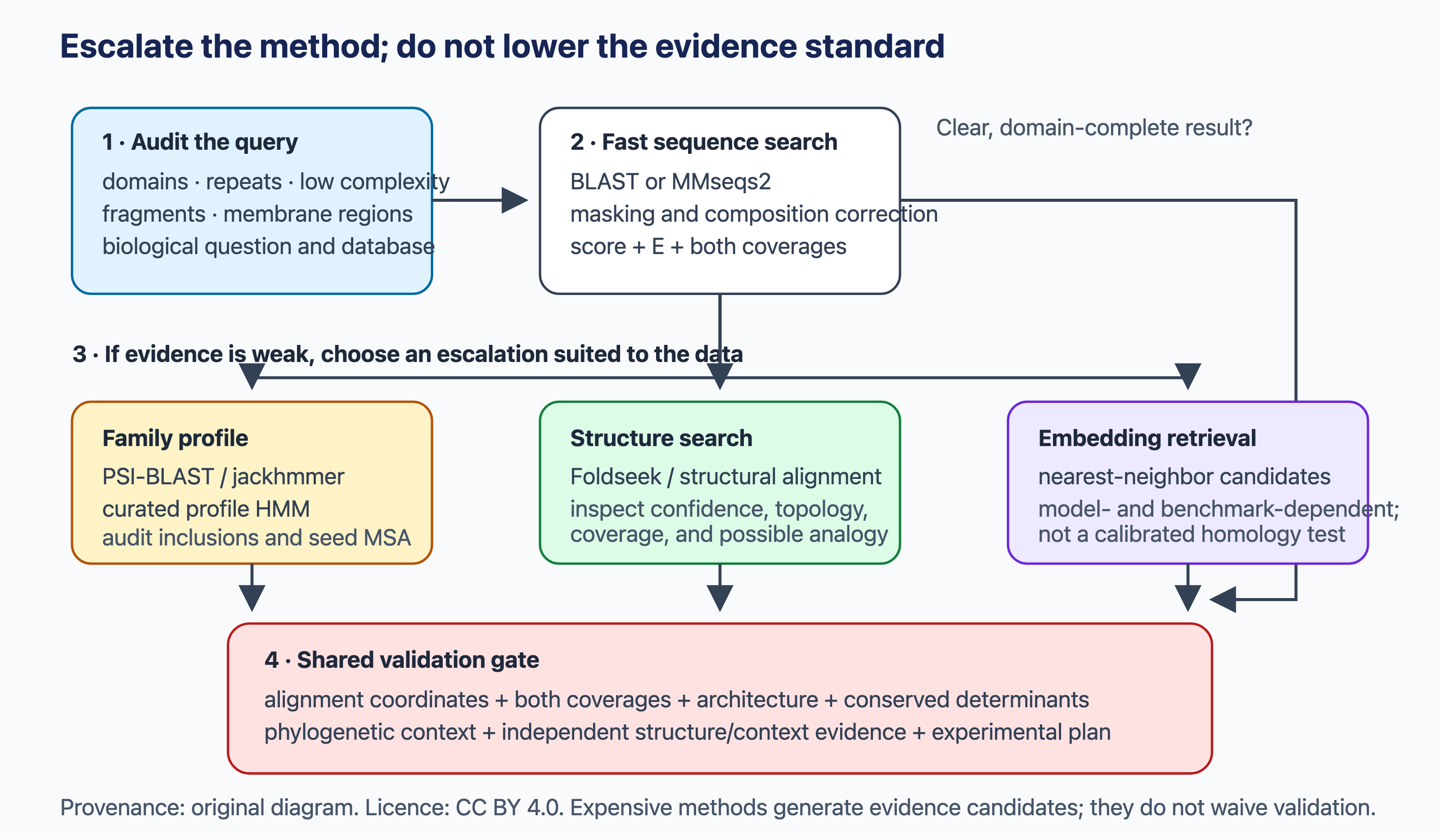
Figure 1.5: A workflow for difficult searches. The query is checked first, and a fast sequence search is run. If the evidence is weak, the search is escalated to profiles, structure or embeddings, depending on the data available. Every candidate, however it was found, then passes the same checks: coordinates and coverage of the alignment, domain architecture, conserved functional residues, phylogenetic context and independent evidence. Figure: Matteo Tadiello, Modern Bioinformatics: From Foundations to Frontiers (CC BY 4.0).

State a conclusion that matches the evidence. Each step from similarity to homology, from homology to orthology, and from orthology to the same detailed function needs more evidence, not a smaller E-value (Chapter 10). Consider a 620-residue bacterial protein whose best hit (\(E = 10^{-35}\), 41% identity) is a eukaryotic enzyme, but where the alignment covers only a central domain of about 230 residues, while the N-terminus is low-complexity and the C-terminus has a transmembrane helix. A defensible annotation is “contains a domain of family F”, and “putative” enzyme only if the catalytic residues are conserved. Copying the name of the top hit to the whole protein is how errors start to propagate through the databases.

Record what was done. The database and its release, the program and its version, and all parameters (matrix, gap costs, masking, E-value and coverage thresholds, and for iterative searches the inclusion threshold of each round) are part of the result. Without them a search cannot be repeated, and its E-values cannot be compared with those of another search.

See also: further explanation in Section D.1.3; related Wikipedia articles in Section E.1.3.

NoteSources

Parts of this section are adapted from the Wikipedia articles BLAST (biotechnology), FASTA, Burrows–Wheeler transform, FM-index, Suffix array and Gumbel distribution (CC BY-SA 4.0, retrieved 2 October 2026). Parts of this section are adapted from Matteo Tadiello, Modern Bioinformatics: From Foundations to Frontiers, chapter “Sequence Alignment and Search Foundations” (CC BY 4.0), used with permission.

1.5 Alignment-free sequence comparison

Every method so far starts from an alignment, or at least from seeds that are extended into one. Alignment has two drawbacks for some problems. First, it is computationally expensive for very long sequences such as whole genomes. Second, it assumes that the two sequences are collinear: homologous positions appear in the same order. That is not true for genomes that have undergone rearrangements, recombination or horizontal gene transfer. Alignment-free methods compare sequences through summary statistics, most often the sets or frequencies of their short words, without computing an alignment at all (Zielezinski et al. 2017).

1.5.1 Word (\(k\)-mer) statistics

The simplest approach represents each sequence by the counts of all its \(k\)-mers, the words of length \(k\). There are \(4^k\) possible \(k\)-mers for DNA and \(20^k\) for proteins. Two sequences are then compared by a distance between their count vectors, for example the Euclidean distance, or the \(D_2\) statistic, which counts the number of shared \(k\)-mer occurrences. Variants correct the counts for what is expected from the composition of shorter words, so that only unexpected word frequencies contribute. The choice of \(k\) matters. A small \(k\) gives words that occur by chance in any sequence. A large \(k\) gives words that are almost never shared once the sequences have diverged. Other families of methods use the lengths of the longest common substrings, matches of spaced words (as in the spaced seeds of Section 1.4), or information-theoretic measures such as how well one sequence compresses given the other.

1.5.2 MinHash and Mash

For large-scale comparisons the most successful idea comes from computer science. The similarity of two sets \(A\) and \(B\), for example the sets of \(k\)-mers of two genomes, can be measured by the Jaccard index \(J = |A \cap B| / |A \cup B|\). Computing it exactly requires storing all \(k\)-mers. MinHash (Broder 1997) estimates it from a small sketch. Every \(k\)-mer is mapped to a number by a hash function, and only the \(s\) smallest hash values of each set are kept, typically \(s = 1000\). The fraction of shared values among the smallest \(s\) values of the union is an unbiased estimate of \(J\). A genome of millions of bases is thus summarised in a few kilobytes, and two sketches are compared in microseconds.

Mash (Ondov et al. 2016) turned this into a tool for genomics. It also converts the Jaccard index into an estimate of the evolutionary distance. Under a simple model in which mutations are independent and each one destroys the \(k\)-mers that overlap it, the Mash distance is

\[ D = -\frac{1}{k} \ln \frac{2J}{1+J}, \]

which approximates the proportion of differing positions (substitutions per site) for closely related sequences. Mash can compare a new genome against all sequenced genomes in seconds, cluster tens of thousands of genomes, or find which known organisms are present in a metagenome.

The same principle of selecting a small, consistent subset of \(k\)-mers appears in other tools of this chapter. Minimizers in minimap2 (Section 1.4) and the \(k\)-mer selection in Linclust are both ways of finding candidate matches without looking at every word.

1.5.3 Applications and limitations

Alignment-free methods are now standard where speed matters more than detail:

  • Species delimitation and genome comparison. The average nucleotide identity (ANI) between two prokaryotic genomes, computed rapidly from matching fragments by tools such as FastANI, shows a clear gap at about 95%, which is widely used as an operational species boundary for bacteria and archaea, although exceptions occur (Jain et al. 2018).
  • Metagenomic classification. Kraken (Wood and Salzberg 2014) assigns each read to a taxon by looking up its \(k\)-mers in a database that maps every \(k\)-mer to the lowest common ancestor of all genomes that contain it. Millions of reads can be classified per minute.
  • Transcript quantification. Pseudo-alignment in tools such as kallisto determines which transcripts a read is compatible with from shared \(k\)-mers, without aligning it base by base (Chapter 7).
  • Phylogenies of many genomes, where the distances are used as input to distance methods such as neighbour joining (Chapter 4).

These measures answer related but different questions, and they should not be confused. The Jaccard index of \(k\)-mer sets (estimated by MinHash) measures how much sequence content two sets share. It depends on \(k\) and is lowered by differences in genome size or gene content even when the shared parts are identical. ANI measures the identity of the shared part only: it is computed over fragments that can be matched, and is reported together with the fraction of each genome that was matched. The Mash distance converts a Jaccard index into an approximate substitution rate, but only under its simple mutation model and only for close relatives. Homology, finally, is a statement about common ancestry (1). A low Jaccard index or the absence of shared \(k\)-mers is not evidence against homology; it usually means only that the sequences have diverged beyond what exact words can detect.

The limitations follow from the method. Exact \(k\)-mer matches disappear quickly as sequences diverge, so alignment-free methods are accurate for closely related sequences, for example within a species or a genus. They are poor at detecting distant homology, where alignment with substitution matrices and profiles is far more sensitive. They also give no alignment, so they cannot say which positions correspond or where the differences are. In practice, the two approaches are complementary. Alignment-free methods are used to decide quickly which sequences to compare, and alignment is used to analyse the comparisons that matter.

See also: further explanation in Section D.1.4; related Wikipedia articles in Section E.1.4.

NoteSources

Parts of this section are adapted from the Wikipedia articles Alignment-free sequence analysis and MinHash (CC BY-SA 4.0, retrieved 2 October 2026).

1.6 Profiles and multiple sequence alignments

Pairwise methods compare one sequence with another. However, homologous sequences rarely come in pairs. A protein usually belongs to a family of tens to millions of related sequences, and the family as a whole carries much more information than any single member. When many homologues are aligned, it becomes visible which positions are invariant (often catalytic or structurally essential residues), which tolerate only certain kinds of amino acid (e.g. only hydrophobic ones in a buried strand), and where insertions and deletions are common (usually surface loops). This section covers how such alignments are built, how short conserved signals (motifs) are described and found, and how the information in an alignment is condensed into a profile that can search databases far more sensitively than a single sequence. The probabilistic version of the profile, the profile hidden Markov model, is described in the next part of this section.

1.6.1 Multiple sequence alignment

What a multiple alignment is

A multiple sequence alignment (MSA) of \(N\) sequences \(S_1, \dots, S_N\) is obtained by inserting gaps into each sequence so that all of them have the same length \(L \ge \max_i |S_i|\). The aligned sequences are written as rows of a matrix, and no column may consist only of gaps. Removing the gaps from a row gives back the original sequence. The intended meaning of a column is that its residues are homologous: they descend from the same position in a common ancestral sequence (1). In practice, a column is a hypothesis of homology. It is most reliable in conserved core regions and least reliable in gap-rich, variable loops.

Multiple alignments are among the most widely used objects in bioinformatics. They are the input to phylogenetic tree reconstruction (Chapter 4). They are used to identify conserved functional residues and sequence motifs, to build profiles and profile HMMs for database search (see the rest of this section and Section 1.9), and to define protein families. They are also central to structure prediction: the coevolution signal that made modern contact and structure prediction possible, including AlphaFold, is extracted from deep MSAs (Chapter 9).

Scoring a multiple alignment

To speak of a “best” alignment, we need an objective function. The most common one is the sum-of-pairs (SP) score. Each column is scored by adding the substitution score for every pair of residues in it, and the alignment score is the sum over columns minus gap penalties:

\[ \mathrm{SP} = \sum_{\text{columns } c} \; \sum_{i<j} s(a_{ic}, a_{jc}), \]

where \(a_{ic}\) is the residue (or gap) of sequence \(i\) in column \(c\) and \(s\) is taken from a substitution matrix such as BLOSUM62 (Section 1.3). Gap–gap pairs are usually scored as zero. Equivalently, the SP score is the sum of the scores of all \(N(N-1)/2\) pairwise alignments induced by the MSA.

The SP score is simple, but it has known weaknesses. It implicitly treats every sequence as equally independent, so a family dominated by many near-identical sequences gives them too much weight. This is why practical methods use sequence weights (see below). It also lacks a sound evolutionary interpretation: in a column with \(N\) copies of the same residue the score grows as \(N^2\), although the evidence comes from a single ancestral residue that has been conserved. Alternative column scores include entropy-based scores, where a column \(c\) with residue frequencies \(p_{a,c}\) is scored by \(H_c = -\sum_a p_{a,c} \log p_{a,c}\) and a good alignment minimises the total entropy. There are also tree-based scores that count the substitutions required on a phylogeny. When alignment programs are compared with reference alignments, two further measures are used. The SP accuracy is the fraction of correctly aligned residue pairs, and the total column (TC) score is the fraction of reference columns that are reproduced exactly.

It is worth stating plainly that there is no single biologically correct objective function for a multiple alignment. The true alignment is defined by evolutionary history (which residues descend from the same ancestral position), and that history is not observed. Every practical method therefore optimises a surrogate: the SP score (progressive methods such as ClustalW), agreement with a library of pairwise alignments (consistency, T-Coffee and the accurate MAFFT modes), expected accuracy under a probabilistic model of alignment (ProbCons, HMM-based aligners), a phylogeny-aware treatment that distinguishes insertions from deletions on a guide tree (PRANK), or agreement with known or predicted structures (structure-aware methods such as 3D-Coffee). These surrogates can disagree, and the “best” alignment under one need not be the best under another. Benchmarks, which use structural superposition as a proxy for homology, are themselves a further surrogate.

Exact alignment is intractable

Dynamic programming (Section 1.3) extends directly from two to \(N\) sequences. Instead of a two-dimensional matrix we fill an \(N\)-dimensional lattice with one axis per sequence. Each cell can be reached from \(2^N - 1\) predecessor cells (every non-empty subset of the sequences advances by one residue). For sequences of length \(L\) this costs \(O(L^N)\) memory and \(O(2^N L^N)\) time. Already three proteins of length 300 need \(2.7 \times 10^7\) cells; ten proteins of that length would need \(\approx 6 \times 10^{24}\).

Two observations made exact methods somewhat more practical. First, Carrillo and Lipman showed in 1988 (Carrillo and Lipman 1988) that the score of each induced pairwise alignment can be bounded using the optimal pairwise alignments. The search can therefore be restricted to the region of the lattice near the intersection of the pairwise optima. The program MSA (Lipman et al. 1989) used this idea to align up to about eight moderately long sequences optimally under the SP score. Second, and more fundamentally, the problem cannot be solved efficiently in general: Wang and Jiang (1994) proved that finding the optimal SP alignment is NP-hard. All widely used MSA programs are therefore heuristics. They give good alignments in practice, but there is no guarantee that they find the optimum of any objective function.

Progressive alignment

The heuristic behind almost all practical MSA programs is progressive alignment, introduced by Feng and Doolittle (1987). The idea is to follow the evolutionary history. Sequences that are closely related can be aligned reliably, so they are aligned first, and the growing alignments are then combined in the order given by an approximate tree. The method has three steps:

  1. Pairwise distances. All \(N(N-1)/2\) pairs are compared, either by full dynamic programming or, for speed, by counting shared short words (\(k\)-tuples). The similarity of each pair is converted into a distance.
  2. Guide tree. A tree is built from the distance matrix with a fast clustering method, typically UPGMA or neighbour joining (Chapter 4). The guide tree is not intended as a phylogeny. It only determines the order in which sequences are joined.
  3. Progressive joining. Following the guide tree from the leaves to the root, sequences and sub-alignments are aligned to each other: sequence to sequence, sequence to alignment, or alignment to alignment. Aligning two alignments (“profile–profile alignment”) is ordinary pairwise dynamic programming in which each “residue” is a column, scored for example by the average substitution score over all residue pairs between the two columns.

Progressive alignment needs only \(O(N^2)\) pairwise comparisons plus \(N-1\) profile alignments, so it scales to thousands of sequences. Its fundamental weakness is greed. Feng and Doolittle stated it as “once a gap, always a gap”: decisions taken early, when two close sequences are aligned, are frozen into the sub-alignment and are never revised when more distant sequences are added. In their method, gaps placed early were replaced by a neutral symbol so that they would not be penalised again. Errors in the early alignments, or in the guide tree, therefore propagate to the final result. This matters most when all sequences are distantly related, because then no reliable early alignments exist.

The Clustal family

The Clustal programs, developed by Des Higgins and colleagues, have been the most widely used implementations of progressive alignment, and two Clustal papers are among the most cited scientific papers of all time.

  • Clustal (1988). The first program (Higgins and Sharp 1988) was written to run on the personal computers of the time. Its name reflects the use of clustering (UPGMA) to build the guide tree, computed from fast \(k\)-tuple similarity scores. ClustalV (1992) was a rewrite in C. It added profile alignment (aligning an alignment to an alignment) and neighbour-joining trees.
  • ClustalW (1994). The W stands for weighting. Thompson et al. (1994) added three improvements that made progressive alignment much more accurate and that remain standard ideas:
    • Sequence weighting. Weights are derived from the branch lengths of the guide tree, so that groups of near-identical sequences are down-weighted and divergent sequences are up-weighted.
    • Varying substitution matrices. The choice of matrix depends on the divergence of the sequences being aligned. Closely related sequences are aligned with “hard” matrices (high-identity BLOSUM or PAM matrices), divergent ones with “soft” ones.
    • Position-specific gap penalties. Gap-opening penalties are reduced in runs of hydrophilic residues, which usually form surface loops, and at positions where the existing alignment already has gaps. They are increased close to existing gaps, so that gaps cluster in the same places instead of being scattered.
    In addition, the joining of very divergent sequences is delayed until the rest of the alignment has been built. ClustalW uses neighbour joining for the guide tree. Because all pairwise distances are computed, the method is \(O(N^2)\) in the number of sequences. ClustalX (1997) added a graphical interface, and Clustal 2 (2007) packaged both.
  • Clustal Omega (2011). By the 2000s, families with tens or hundreds of thousands of members had become common, and computing all pairwise distances was no longer feasible. Clustal Omega (Sievers et al. 2011) replaced the core of the method:
    • Guide trees are computed with mBed. Each sequence is represented by its distances to a small set of “seed” sequences (an embedding in a low-dimensional space). The sequences are clustered (k-means) in that space, and a UPGMA tree is built within clusters. This reduces the cost from \(O(N^2)\) to \(O(N \log N)\).
    • The progressive joining step uses HHalign from the HH-suite. Each sub-alignment is turned into a profile hidden Markov model, and the two HMMs are aligned, which is more sensitive than simple profile–profile scoring.
    As a result, Clustal Omega can align more than 100,000 sequences on a single processor in a few hours, while keeping accuracy comparable to the best methods on small benchmarks. Its authors also stressed that alignment accuracy decreases when very many sequences are aligned with most methods, and that big alignments need methods designed for them.

Consistency and iterative refinement

Two further ideas address the greediness of progressive alignment.

Consistency. If residue \(x\) in sequence A aligns with residue \(y\) in sequence C, and \(y\) aligns with residue \(z\) in B, then the pairwise alignment of A and B should preferably align \(x\) with \(z\). T-Coffee (Notredame et al. 2000) uses this transitivity. It first computes a primary library of pairwise alignments of all pairs, using both global alignments (from ClustalW) and local ones (from LALIGN). Each aligned residue pair is weighted by the identity of the alignment it came from. The library is then extended: the weight of a pair \((x, z)\) is increased by the support from every third sequence C through which \(x\) and \(z\) are consistently aligned. Finally, an ordinary progressive alignment is carried out, but using the extended library weights instead of a substitution matrix as the scores. Information from all sequences thus influences every pairwise step, and errors made early are much less likely. The cost is time and memory that grow as \(O(N^3 L^2)\), which limits T-Coffee to at most a few hundred sequences. Consistency is also the basis of probabilistic aligners such as ProbCons, and of the most accurate modes of MAFFT.

Iterative refinement. An alignment can be improved after it has been built. A typical refinement step divides the sequences into two groups (for example by deleting one edge of the guide tree), realigns the two sub-alignments to each other, and keeps the result if the objective score improves. MUSCLE (Edgar 2004) combines progressive alignment with such refinement in three stages:

  1. A draft progressive alignment using fast \(k\)-mer distances and a UPGMA tree.
  2. An improved progressive alignment: the tree is rebuilt from the (Kimura-corrected) identities of the draft alignment, and the alignment is recomputed for the parts of the tree that changed.
  3. Refinement by tree-dependent restricted partitioning: edges of the tree are deleted in turn, the two resulting profiles are realigned, and the change is accepted if the score improves.

MUSCLE scores profile columns with a “log-expectation” function, and it was notable for being both faster and more accurate than ClustalW and T-Coffee on the benchmarks of the time.

MAFFT, first published by Kazutaka Katoh and colleagues in 2002 (Katoh et al. 2002; Katoh and Standley 2013), introduced a different speed-up for the pairwise step. Each amino acid is represented by numerical values of its volume and polarity. The correlation between two sequences at every possible relative offset can then be computed with the fast Fourier transform (FFT) in \(O(L \log L)\) time. Peaks in this correlation reveal homologous segments, and dynamic programming is restricted to the regions between them. MAFFT offers a range of strategies. FFT-NS-2 is a fast progressive method. FFT-NS-i adds iterative refinement. L-INS-i, G-INS-i and E-INS-i are consistency-based iterative methods using local, global or generalised pairwise alignments, and they are among the most accurate methods available for up to a few hundred sequences. Modern versions also include options for very large data sets and for adding new sequences to an existing alignment.

How good are multiple alignments?

Because the true alignment is unknown, MSA methods are evaluated on reference alignments in which the correct homologous positions are believed to be known. The most widely used benchmarks, such as BAliBASE (Thompson et al. 1999), derive the reference from superpositions of known three-dimensional structures, since structurally equivalent residues are the best available proxy for homologous ones. Methods are compared by the SP accuracy and the TC score defined above. Three conclusions have held for decades:

  • For sequences above about 30–40% identity, all good methods agree and are essentially correct. Below about 20–25% identity (the “twilight zone”,
    1. all methods make many errors, and the differences between them become large.
  • Consistency-based and iterative methods are the most accurate on small and medium-sized sets. Clustal Omega and the fast modes of MAFFT are the practical choices for very large sets.
  • Alignment errors are concentrated in loops and at the ends of sequences. They can affect downstream analyses, for example phylogenetic trees (Chapter 4), so variable regions are often removed (“trimmed”) before tree building. Phylogeny-aware aligners such as PRANK (Löytynoja and Goldman 2008) treat insertions and deletions more realistically than methods that systematically minimise the number of gaps.

Alignment uncertainty

A multiple alignment is an estimate, but it is usually used as if it were data. A tree, a conservation score or a profile built from it inherits its errors, and nothing in a single alignment shows which columns are reliable. Different programs, different guide trees and even different input orders can give different alignments of the same sequences, and the differences are concentrated in exactly the divergent regions that matter most for remote homology and deep phylogeny.

One response is to make the uncertainty visible. MUSCLE5 (Edgar 2022) builds an ensemble of alignments by perturbing the guide tree and the scoring parameters. The fraction of ensemble members in which a column, or a whole downstream result such as a branch of a tree, is recovered is a measure of its confidence. Its benchmarks also showed that a single confident-looking alignment can hide considerable uncertainty, and that conclusions which change between equally plausible alignments should not be trusted. Consistency-based aligners such as T-Coffee and probabilistic aligners can likewise report a reliability score for each column.

Trimming (removing unreliable columns) is a related choice. It can reduce noise, but it also removes fast-evolving positions that carry real signal (Section 4.4). Whether and how to trim is therefore a modelling decision, best tested by checking whether the conclusion changes.

1.6.2 Sequence motifs

A sequence motif is a short, recurring pattern in DNA, RNA or protein sequences that is assumed to have a biological function. Examples are transcription factor binding sites in DNA, splice signals in RNA, and in proteins, catalytic sites, metal-binding sites, sorting signals and sites of post-translational modification. Motifs are often only 5–20 residues long. They may lie in otherwise unrelated sequences: regulatory sites in promoters are not, in general, homologous to each other. Such sites may have arisen independently many times, because only the binding specificity of the protein recognising them is conserved (1). Short protein motifs such as phosphorylation sites can also arise by convergence.

Consensus sequences and patterns

The simplest description of a motif is a consensus sequence: the most common residue at each position, for example TATAAT for the bacterial promoter \(-10\) box (the “Pribnow box”). A consensus discards the information about how variable each position is. Very few real sites actually match the consensus exactly.

A more expressive description is a pattern, written as a regular expression. The PROSITE database, created by Amos Bairoch in 1988 (Bairoch 1991; Sigrist et al. 2012), made such patterns standard for proteins. In PROSITE notation:

  • elements are separated by -;
  • x means any residue;
  • [ST] means S or T;
  • {P} means any residue except P;
  • x(2,4) means between two and four arbitrary residues;
  • < and > anchor the pattern to the N- or C-terminus.

Three well-known examples:

Motif PROSITE pattern
N-glycosylation site N-{P}-[ST]-{P}
ATP/GTP-binding P-loop (Walker A) [AG]-x(4)-G-K-[ST]
C2H2 zinc finger C-x(2,4)-C-x(3)-[LIVMFYWC]-x(8)-H-x(3,5)-H

Patterns are easy to read and to search for. However, matching is binary: a sequence either matches or it does not. Every allowed residue counts the same, however rare it is at that position, and a single unusual residue causes a miss. Short patterns also match many sequences by chance; the N-glycosylation pattern is found in most proteins, while only a minority of the matches are real glycosylation sites. PROSITE therefore documents the expected numbers of true and false matches for each pattern. For divergent families it uses profiles (below) instead.

Position weight matrices

A position weight matrix (PWM), also called a position-specific scoring matrix (PSSM), assigns a score to every residue at every position of a gap-free motif of length \(w\). It is built from a set of aligned sites in three steps:

  1. Counts. \(n_{b,j}\) is the number of sites with residue \(b\) at position \(j\) (the position frequency matrix).
  2. Probabilities. These are estimated with pseudocounts, which prevent residues that are absent from a small training set from getting probability zero (and a score of \(-\infty\)): \[ p_{b,j} = \frac{n_{b,j} + \alpha_b}{N + \sum_{b'} \alpha_{b'}}, \] where \(N\) is the number of sites and \(\alpha_b\) the pseudocount for residue \(b\).
  3. Log-odds weights. The probabilities are compared with a background model \(q_b\), typically the overall base or amino acid composition: \[ W_{b,j} = \log_2 \frac{p_{b,j}}{q_b}. \]

The score of a candidate site \(x_1 \dots x_w\) is the sum of the weights, \(\sum_j W_{x_j, j}\). It is the log-likelihood ratio between “this is an instance of the motif” and “this is background sequence”, under the assumption that positions are independent. A score above zero means the site is more likely under the motif model than under the background. In practice, a threshold is set to balance true and false matches, as for the substitution scores of Section 1.3, which are log-odds scores of the same kind. For DNA-binding proteins, the PWM score is also approximately proportional to the binding energy, which gives the model a physical interpretation (Stormo 2000).

Worked example (illustrative data):

Ten aligned sites (illustrative): TATAAT, TATAAT, TAAAAT, TATACT, GATAAT, TATGAT, TACAAT, TATATT, AATAAT, TATAAG.

Counts (position frequency matrix):

1 2 3 4 5 6
A 1 10 1 9 8 0
C 0 0 1 0 1 0
G 1 0 0 1 0 1
T 8 0 8 0 1 9

Log-odds weights \(W_{b,j} = \log_2 (p_{b,j}/q_b)\) in bits, with a pseudocount of 0.25 per base and a uniform background \(q_b = 0.25\):

1 2 3 4 5 6
A -1.14 +1.90 -1.14 +1.75 +1.58 -3.46
C -3.46 -3.46 -1.14 -3.46 -1.14 -3.46
G -1.14 -3.46 -3.46 -1.14 -3.46 -1.14
T +1.58 -3.46 +1.58 -3.46 -1.14 +1.75

Information content per position (bits, from the raw frequencies): 1.08, 2.00, 1.08, 1.53, 1.08, 1.53; total 8.3 bits.

Scores of three test sequences (sum of the weights at each position):

Sequence Score (bits)
TATAAT (consensus) +10.15
TACGAT +4.54
GCGCGC -18.43

The consensus TATAAT gets the highest possible score. TACGAT, which differs at two positions, still gets a clearly positive score. A GC-rich sequence gets a strongly negative score.

How much a motif stands out from the background is measured by its information content. For position \(j\) it is the relative entropy (Kullback–Leibler divergence) between the motif and the background distributions:

\[ I_j = \sum_b p_{b,j} \log_2 \frac{p_{b,j}}{q_b}. \]

With a uniform background this is \(I_j = \log_2 |\mathcal{A}| - H_j\), where \(H_j\) is the Shannon entropy of the column and \(|\mathcal{A}|\) is the alphabet size. The maximum is therefore 2 bits for DNA and \(\log_2 20 \approx 4.3\) bits for proteins. Sequence logos (Schneider and Stephens 1990) display this graphically: the height of the stack at each position is \(I_j\), and each letter’s height is proportional to its frequency (Figure 1.6). For small samples a correction term is usually subtracted, because entropy estimated from few sequences is biased downwards.
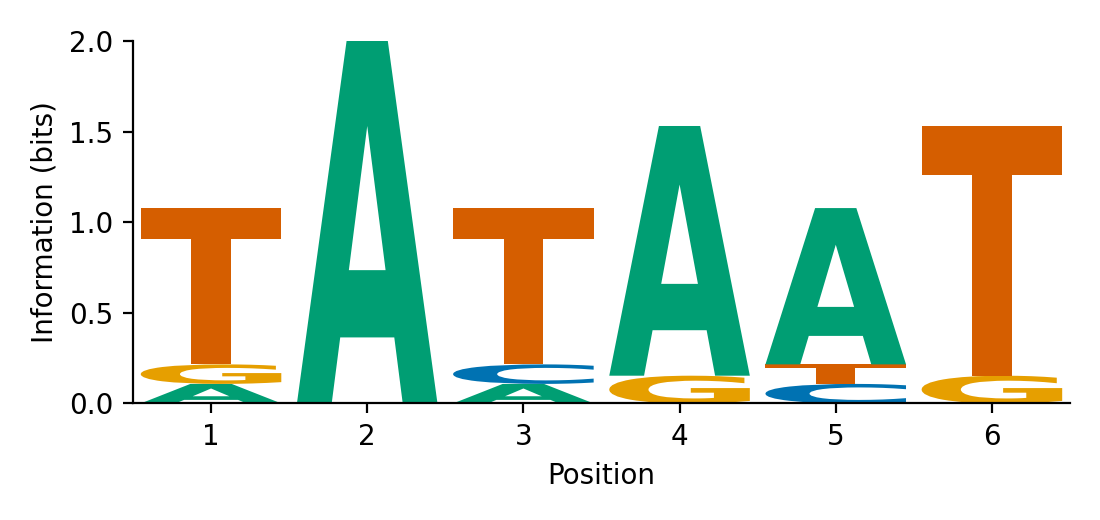
The total information content of a motif also says how often it is expected to occur by chance. A motif with \(I\) bits matches a random sequence about once every \(2^I\) positions. The 8.3 bits of the example above therefore correspond to one chance match every few hundred base pairs, which is why real promoters are recognised by combinations of signals, not by the \(-10\) box alone.

PWMs assume that positions contribute independently and that motifs have no insertions or deletions. Models with dependencies between positions exist. Allowing insertions and deletions leads to profile HMMs, described later in this section.

Finding motifs de novo

Often the sites are not known in advance. We may have, for example, a set of promoters of co-regulated genes and want to find the motif that they share. This motif-finding problem can be stated as follows. Given \(N\) sequences, find one site of width \(w\) in each (or in most), such that the sites are as similar to each other as possible, for example as measured by the information content of the resulting PWM. The search space is huge (about \(L^N\) combinations of starting positions for sequences of length \(L\)), so stochastic and statistical methods are used.

Gibbs sampling (Lawrence et al. 1993) is a Markov chain Monte Carlo method. The algorithm is:

  1. Choose a random starting position \(a_i\) for a site in each sequence \(i\).
  2. Choose one sequence \(z\) and remove it.
  3. Build a PWM (with pseudocounts) from the current sites in the remaining \(N-1\) sequences.
  4. For every possible position \(x\) in sequence \(z\), compute the ratio \(Q_x / P_x\). Here \(Q_x\) is the probability of the \(w\)-long segment starting at \(x\) under the PWM, and \(P_x\) its probability under the background model.
  5. Sample a new site position \(a_z\) with probability proportional to \(Q_x/P_x\), i.e. randomly rather than greedily.
  6. Repeat from step 2 until the motif stops improving.

Because the new position is sampled rather than chosen as the best, the algorithm can escape from poor local optima, and it gradually converges on a strong shared motif if one exists. Lawrence and colleagues also introduced “phase shift” moves, which shift all sites a few positions left or right, because the sampler otherwise tends to get stuck on a shifted version of the true motif. Gibbs sampling was originally applied to find subtle shared motifs in sets of weakly similar proteins, but it became particularly popular for transcription factor binding sites.

MEME (Multiple EM for Motif Elicitation; Bailey and Elkan (1994)) uses the expectation–maximisation (EM) algorithm instead. The data are modelled as a mixture of motif occurrences, described by a PWM, and background sequence. EM alternates two steps:

  • E-step: for every position in every sequence, compute the posterior probability that a motif occurrence starts there, given the current PWM.
  • M-step: re-estimate the PWM as a weighted average over all positions, weighted by those probabilities.

Each iteration cannot decrease the likelihood, so EM converges, but only to a local optimum. MEME therefore starts EM from many initial PWMs built from substrings that actually occur in the data, and keeps the best result. After a motif is found, its occurrences are down-weighted and the search is repeated to find further motifs. MEME also made the model of how many sites a sequence contains explicit:

  • OOPS: exactly one occurrence per sequence;
  • ZOOPS: zero or one occurrence per sequence;
  • TCM (two-component mixture): any number of occurrences.

Each motif is reported with an E-value for its significance, and the companion program MAST searches databases with the discovered motifs.

Both approaches have the same basic limitations. They need the motif width in advance (or try several), and they find statistically over-represented patterns, which may include repeats or low-complexity sequence as well as functional sites. A motif found de novo is a hypothesis, which needs support from experiments or from conservation across species.

1.6.3 Profiles: from patterns to position-specific scoring

PROSITE patterns versus profiles

The limitations of patterns, together with the observation that the conserved positions of a family are far more informative than the variable ones, led to profiles. Gribskov et al. (1987) defined a profile as a position-specific scoring table derived from a multiple alignment. It has one row for each alignment position, with a score for each of the 20 amino acids and a position-specific penalty for opening and extending gaps. A query sequence is aligned to the profile by ordinary dynamic programming, using the profile row instead of a fixed substitution score at each position.

In Gribskov’s construction, the score for amino acid \(b\) at position \(j\) is an average of substitution-matrix scores, weighted by the residues seen in the alignment column: \(W_{b,j} = \sum_a f_{a,j}\, s(a, b)\). Here \(f_{a,j}\) is the frequency of residue \(a\) in column \(j\) and \(s\) is a substitution matrix such as PAM250. This simple formula already has the crucial property that a residue never seen at a position, but similar to those that are, still scores well. The profile therefore generalises beyond the sequences it was built from.

The differences from a pattern can be summarised as:

Pattern (regular expression) Profile
Representation Allowed residues per position Score for every residue at every position
Matching Yes/no Graded score; significance estimated
Insertions/deletions Fixed ranges such as x(2,4) Position-specific gap penalties
Rare but allowed residues Weighted like common ones Lower score
Best suited for Short, highly conserved sites Whole domains and divergent families

PROSITE added such “generalised profiles” in the 1990s to cover families that patterns could not describe (Sigrist et al. 2012). The profile idea is also the basis of PSI-BLAST and, in probabilistic form, of the profile HMMs in Pfam (Section 1.9).

Building a good profile

How well a profile works depends on how it is estimated. Three issues recur in all profile methods, including profile HMMs:

  • Sequence weighting. Sequence databases are very redundant. If a family alignment contains 50 nearly identical sequences from one subfamily and five divergent ones, unweighted frequencies describe that subfamily, not the family. Weighting schemes give less weight to sequences that are similar to many others. A widely used simple scheme is the position-based weighting of Henikoff and Henikoff (Henikoff and Henikoff 1994). In each column with \(r\) different residue types, a sequence whose residue occurs \(s\) times receives \(1/(rs)\), and these contributions are summed over all columns. ClustalW’s tree-based weights serve the same purpose.
  • Pseudocounts and priors. A column with few sequences, or few effective sequences after weighting, gives unreliable frequencies. Pseudocounts are added to fill in residues that have not been observed. Better than uniform pseudocounts are ones that use what we know about amino acid substitutions. One option is to derive them from a substitution matrix: residues similar to those observed get more pseudocounts. Another is Dirichlet mixture priors (Sjölander et al. 1996), which encode typical kinds of alignment columns (“hydrophobic”, “small”, “aromatic”, …) learnt from many alignments. The fewer the sequences, the more the estimate relies on the prior.
  • Position-specific gaps. Insertions and deletions are frequent in loops and rare in the core. Profiles that use lower gap penalties where the training alignment has gaps align new sequences more accurately.

A worked PSSM

A small example shows how the pieces fit together (Figure 1.7). Let column \(i\) of an alignment contain \(n_i(a)\) copies of amino acid \(a\) and \(N_i\) residues in total (gaps are not counted), and let \(p(a)\) be the background frequency of \(a\). With a pseudocount of total weight \(\alpha\), distributed in proportion to the background, the estimated frequency and the score in bits are

\[ \hat q_i(a) = \frac{n_i(a) + \alpha\, p(a)}{N_i + \alpha}, \qquad w_i(a) = \log_2 \frac{\hat q_i(a)}{p(a)}. \]

Take the six aligned sequences ADKLG, ADKLG, AEKLG, ADQLG, -DKLG and ADKIG, and \(\alpha = 1\). Column 2 has five D and one E. With \(p(\text{D}) = 0.059\), \(\hat q_2(\text{D}) = (5 + 0.059)/7 = 0.72\) and \(w_2(\text{D}) = \log_2(0.72/0.059) = +3.6\) bits. With \(p(\text{E}) = 0.058\), E scores \(+1.4\) bits. A residue not seen in the column, such as A, gets \(\hat q_2(\text{A}) = p(\text{A})/7\) and therefore \(\log_2(1/7) = -2.8\) bits: a penalty, but not the \(-\infty\) that raw frequencies would give. (With this simple background-weighted pseudocount, every unobserved residue gets the same score; a substitution-matrix or Dirichlet prior would penalise I less than W in a column of L, for example.) The score of an ungapped sequence segment \(x_1 \ldots x_L\) is the sum \(\sum_i w_i(x_i)\), one cell per column. A positive sum does not by itself mean that the sequence belongs to the family: as for any score, a threshold or an E-value must be calibrated, and gaps need their own model.
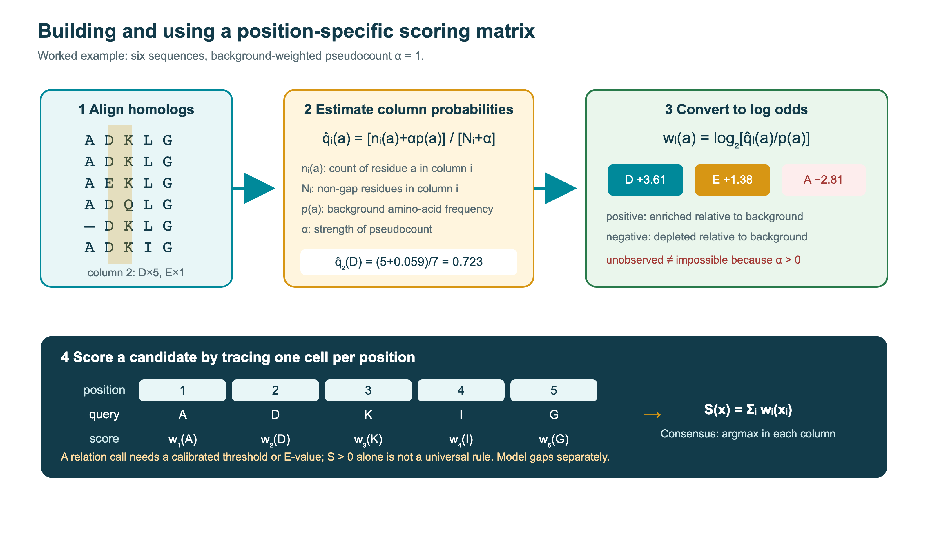
Figure 1.7: Building and using a position-specific scoring matrix for the six-sequence example in the text: (1) count residues in each column of the alignment, (2) estimate column frequencies with background-weighted pseudocounts, (3) convert them to log-odds scores in bits, and (4) score a new sequence by adding one cell per position. Figure: Matteo Tadiello, Modern Bioinformatics: From Foundations to Frontiers (CC BY 4.0).

PSI-BLAST

PSI-BLAST (Position-Specific Iterated BLAST; Altschul et al. (1997)) made profile searching fast, automatic and widely used. It builds a profile from its own search results, without a pre-made family alignment:

  1. Round 1 is an ordinary BLAST search (Section 1.4) of the query against a large database such as UniRef or NCBI nr.
  2. All hits with an E-value below an inclusion threshold (typically 0.001–0.005) are collected into a multiple alignment, which is anchored on the query (columns where the query has a gap are ignored).
  3. A PSSM with one column per query position is computed from this alignment. The sequences are weighted to reduce redundancy, and pseudocounts are derived from the BLOSUM62 matrix. The amount of pseudocount decreases as the number of effectively independent sequences grows.
  4. The PSSM replaces the query and the substitution matrix in the next search round. BLAST’s word seeding, extension and Karlin–Altschul statistics work unchanged with position-specific scores.
  5. Steps 2–4 are repeated for a fixed number of iterations, or until no new sequences are found (“convergence”).

Each round, the profile represents the family better than the query alone did, so homologues too distant to be found in the first round can be found in later ones. In a benchmark based on structurally classified domains in SCOP, Park et al. (1998) showed that profile methods (PSI-BLAST and the HMM-based SAM-T98) detected about three times as many remote homologues as pairwise methods (BLAST, FASTA and Smith–Waterman) at the same error rate. This was one of the clearest demonstrations of the value of family information, and PSI-BLAST profiles became the standard input to secondary structure, contact and fold prediction methods in the 1990s and 2000s (Chapter 9).

The iteration also has a well-known failure mode, profile corruption (also called profile drift). If a single unrelated sequence passes the inclusion threshold, perhaps through a low-complexity region, a coiled coil or a promiscuous domain shared with the query, it is included in the profile. In the next round it pulls in its own relatives, and after a few iterations the profile may describe a different family. The E-values of the later rounds are then misleading, because they measure similarity to the corrupted profile, not to the original query. The same problem affects every iterative profile search, including jackhmmer, HHblits and MMseqs2 profile searches.

Corruption can often be recognised by inspecting the rounds rather than only the final list. Warning signs are a sudden jump in the number of hits from one round to the next; new hits that align only to a short part of the query, such as a single low-complexity segment, coiled coil or repeat; and hits whose annotations belong to a clearly different family. Several things reduce the risk:

  • a strict inclusion threshold;
  • masking low-complexity regions;
  • composition-based statistics, which correct scores for sequences with unusual amino acid composition (Schäffer et al. 2001);
  • checking that new hits are plausible;
  • limiting the number of iterations.

A second limitation is that PSI-BLAST, like BLAST, uses ad hoc gap penalties and treats the profile as a series of independent columns. The probabilistic framework of hidden Markov models, which models insertions and deletions position by position and calculates significance in a principled way, addresses both of these points. It is the subject of the next part of this section.

See also: further explanation in Section D.1.5; related Wikipedia articles in Section E.1.5.

NoteSources

Parts of this section are adapted from the Wikipedia articles Multiple sequence alignment, Clustal, Sequence motif, Position weight matrix, Sequence logo, Gibbs sampling, Expectation–maximization algorithm, PROSITE and BLAST (biotechnology) (CC BY-SA 4.0, retrieved 2 October 2026). Parts of this section are adapted from Matteo Tadiello, Modern Bioinformatics: From Foundations to Frontiers, chapter “Sequence Alignment and Search Foundations” (CC BY 4.0), used with permission.

1.6.4 Hidden Markov models

Position-specific scoring matrices and PSI-BLAST profiles score each column of a family independently, and they treat insertions and deletions with ad hoc, position-independent gap penalties. Hidden Markov models (HMMs) put the whole idea of a profile on a probabilistic footing. Substitutions, insertions and deletions all become probabilities that can be estimated from data, and an alignment of a sequence to a family becomes a path through a probabilistic model. The same small set of dynamic programming algorithms then gives the best alignment, the total probability of the sequence, and the confidence of every aligned residue. HMMs are the basis of HMMER, Pfam and the HH-suite. They are also used, under other names, for gene finding (Chapter 5) and membrane-protein topology prediction (Chapter 9). They are the most important probabilistic model in sequence bioinformatics. The textbook treatment is Durbin et al. (1998); short introductions are Eddy (2004a) and Rabiner (1989).

From Markov chains to hidden Markov models

A Markov chain is a sequence of random variables \(x_1, x_2, \ldots, x_L\) in which the probability of each symbol depends only on the previous one:

\[ P(x) = P(x_1)\prod_{i=2}^{L} P(x_i \mid x_{i-1}) = P(x_1)\prod_{i=2}^{L} a_{x_{i-1}x_i}. \]

The transition probabilities \(a_{st}\) form a matrix whose rows sum to one. A first-order Markov chain over the four nucleotides can, for example, capture the fact that CG dinucleotides are rare in most of the human genome (the C is often methylated and mutates to T). It can also capture that they are more common in CpG islands near promoters. Two such chains, one trained on islands and one on background, can be used to classify a given stretch of DNA by the log-odds ratio of the two models (Durbin et al. 1998).

Classification of a given stretch is not the real problem, however. In a chromosome we do not know where the islands start and end. A hidden Markov model solves this by separating what we observe from what we want to infer. An HMM has:

  • a set of hidden states \(k = 1, \ldots, N\) (for example “island” and “background”, or “exon”, “intron” and “intergenic”);
  • transition probabilities \(a_{kl} = P(\pi_i = l \mid \pi_{i-1} = k)\) between states, where \(\pi = \pi_1 \ldots \pi_L\) is the state path. The path itself is a Markov chain;
  • emission probabilities \(e_k(b) = P(x_i = b \mid \pi_i = k)\), the probability of observing symbol \(b\) when the model is in state \(k\);
  • start (and optionally end) probabilities, often written as transitions \(a_{0k}\) from a silent begin state 0.

The observed sequence is generated by walking along the state path and emitting one symbol from each state. The joint probability of a sequence \(x\) and a path \(\pi\) is simply the product of all transitions and emissions used:

\[ P(x, \pi) = a_{0\pi_1} \prod_{i=1}^{L} e_{\pi_i}(x_i)\, a_{\pi_i \pi_{i+1}}, \]

with \(a_{\pi_L\pi_{L+1}}\) the transition to the end state (or 1 if there is no end state). The model is “hidden” because many different paths can generate the same observed sequence, and in general we only see \(x\).

The standard teaching example, from Durbin et al. (1998), is the occasionally dishonest casino. A casino uses a fair die most of the time, but occasionally switches to a loaded die that shows a six half of the time. We observe only the rolls. The hidden states are Fair (F) and Loaded (L), with emission probabilities \(e_F(b) = 1/6\) for all faces, \(e_L(6) = 0.5\) and \(e_L(b) = 0.1\) for \(b = 1, \ldots, 5\). The transition probabilities are \(a_{FL} = 0.05\) and \(a_{LF} = 0.1\). The model is used as a worked example below.

History

Hidden Markov models were described by Leonard Baum and colleagues at the Institute for Defense Analyses in Princeton in a series of statistical papers from 1966 to the early 1970s. These included the estimation algorithm now called the Baum–Welch algorithm, developed by Baum and Lloyd Welch (Baum et al. 1970). Independently, Andrew Viterbi published in 1967 the dynamic-programming decoding algorithm for convolutional codes in noisy communication channels that now carries his name (Viterbi 1967). The Viterbi algorithm has a history of multiple invention. It is essentially the same recursion that Needleman and Wunsch used for alignment (Section 1.3), and at least seven independent discoveries have been documented.

The first major application was speech recognition, from James Baker’s work in 1975 and Frederick Jelinek’s group at IBM, where the hidden states are phonemes or words and the observations are acoustic features. Lawrence Rabiner’s 1989 tutorial (Rabiner 1989) became the standard introduction and brought the methods to a wide audience. In the second half of the 1980s HMMs began to be used to segment DNA, for example by base composition (Churchill 1989). In the early 1990s David Haussler’s group in Santa Cruz, with Anders Krogh, introduced profile HMMs for protein families (Krogh et al. 1994). Within a few years HMMs were used for gene finding (GENSCAN, GeneMark.hmm; Burge and Karlin (1997); Lukashin and Borodovsky (1998)), transmembrane topology prediction (TMHMM; Krogh et al. (2001)), signal peptides and many other problems. Sean Eddy’s 1998 review of profile HMMs (Eddy 1998) and the textbook by Durbin, Eddy, Krogh and Mitchison (Durbin et al. 1998) made them standard bioinformatics tools.

The three (four) problems

Rabiner formulated the use of an HMM as three basic problems. Biology adds a fourth, posterior decoding, which turns out to be very important.

Problem Question Algorithm
Evaluation What is the probability \(P(x)\) of the sequence, summed over all paths? Forward
Decoding Which single path \(\pi^*\) is most probable? Viterbi
Posterior decoding What is the probability that residue \(i\) was emitted by state \(k\)? Forward–backward
Learning Which parameters \(a_{kl}, e_k(b)\) make the training data most probable? Baum–Welch (EM), Viterbi training

The naive solution to the first two problems is to enumerate all paths, but there are \(N^L\) of them. All the algorithms below avoid this by dynamic programming over the sequence positions. They use the fact that, because of the Markov property, the best (or summed) way to reach state \(l\) at position \(i+1\) only depends on the values for all states at position \(i\).

Viterbi: the most probable path

Let \(v_k(i)\) be the probability of the most probable path that ends in state \(k\) after emitting \(x_1 \ldots x_i\). Then

\[ v_l(i+1) = e_l(x_{i+1}) \max_k \big( v_k(i)\, a_{kl} \big), \qquad v_k(1) = a_{0k}\, e_k(x_1). \]

For each cell we store a traceback pointer to the \(k\) that gave the maximum. The probability of the best path is \(P(x, \pi^*) = \max_k v_k(L) a_{k0}\), and the path itself is recovered by following the pointers back from the best final state. This is exactly the structure of the alignment recursions in Section 1.3: a table filled from left to right, a max over predecessors, and traceback.

Forward: the probability of the sequence

If we replace the maximum by a sum, we obtain the probability of the sequence summed over all paths. Let \(f_k(i) = P(x_1 \ldots x_i, \pi_i = k)\). Then

\[ f_l(i+1) = e_l(x_{i+1}) \sum_k f_k(i)\, a_{kl}, \qquad P(x) = \sum_k f_k(L)\, a_{k0}. \]

\(P(x)\) is what we want when we ask whether a sequence belongs to a family. It does not depend on choosing one particular alignment, and it is the natural quantity to compare with a null model.

Backward and posterior decoding

The backward variable \(b_k(i) = P(x_{i+1} \ldots x_L \mid \pi_i = k)\) is computed by the same kind of recursion, from the end of the sequence:

\[ b_k(i) = \sum_l a_{kl}\, e_l(x_{i+1})\, b_l(i+1), \qquad b_k(L) = a_{k0}. \]

Combining the two gives the posterior probability that residue \(i\) was emitted by state \(k\), given the whole sequence:

\[ P(\pi_i = k \mid x) = \frac{f_k(i)\, b_k(i)}{P(x)}. \]

Posterior decoding chooses, at each position, the state with the highest posterior probability. It can give a better per-residue accuracy than the Viterbi path, but the resulting sequence of states is not guaranteed to be a valid path (it may use a transition with zero probability). More importantly, the posteriors measure how certain each part of the result is. In profile HMM alignments they tell which aligned residues are reliable and which are essentially guesses. HMMER reports them under each alignment.

Complexity and numerical issues

For an HMM with \(N\) states and a sequence of length \(L\), all three algorithms need \(O(N^2L)\) time, because every cell considers every predecessor state, and \(O(NL)\) memory. If the model has a sparse transition structure, as profile HMMs do, the time is proportional to the number of non-zero transitions, \(O(NL)\) for a profile. The Viterbi path can be found in linear memory with the same divide-and-conquer trick used for pairwise alignment (Hirschberg; Myers and Miller (1988)).

The probabilities quickly become smaller than the smallest number a computer can represent: a product of a few hundred probabilities below 0.1 underflows double precision. Viterbi is therefore computed in log space, where products become sums and the maximum is unchanged. The forward and backward algorithms need sums of probabilities. They are computed either with scaling (normalising the column at each position and keeping track of the scaling factors, as in Rabiner (1989)) or in log space with the identity \(\log(e^a + e^b) = \max(a,b) + \log\big(1 + e^{-|a-b|}\big)\), often implemented with a lookup table.

Learning the parameters

If the state paths of the training sequences are known (for example, annotated genes, or sequences in a curated multiple alignment), the maximum-likelihood parameters are just normalised counts: \(a_{kl} = A_{kl} / \sum_{l'} A_{kl'}\) and \(e_k(b) = E_k(b) / \sum_{b'} E_k(b')\), where \(A\) and \(E\) count the transitions and emissions used. Pseudocounts or priors are added to avoid zero probabilities for events that happen not to be observed.

If the paths are unknown, the Baum–Welch algorithm estimates the parameters iteratively. It is a special case of the expectation–maximisation (EM) algorithm. In the E step, the forward and backward variables give the expected number of times each transition and emission is used, given the current parameters:

\[ A_{kl} = \sum_j \frac{1}{P(x^j)} \sum_i f^j_k(i)\, a_{kl}\, e_l(x^j_{i+1})\, b^j_l(i+1), \qquad E_k(b) = \sum_j \frac{1}{P(x^j)} \sum_{i:\,x^j_i = b} f^j_k(i)\, b^j_k(i). \]

In the M step, these expected counts replace the observed counts in the formulas above. Each iteration is guaranteed not to decrease the likelihood of the training data, but the algorithm converges to a local maximum, so the result depends on the starting point. A cheaper alternative is Viterbi training: align all sequences with the current model, count the transitions and emissions on the Viterbi paths, and re-estimate. It optimises the probability of the best paths rather than the full likelihood, and is often used in practice. HMMs can also be trained discriminatively, or with Bayesian priors on the parameters, for example Dirichlet distributions (see below).

Worked example: the dishonest casino

To see the algorithms at work, 300 rolls were simulated from the casino model above, and the Viterbi and forward–backward algorithms were then run on the observed rolls only. Figure 1.8 shows the true (hidden) states, the Viterbi path, and the posterior probability that each roll came from the loaded die.
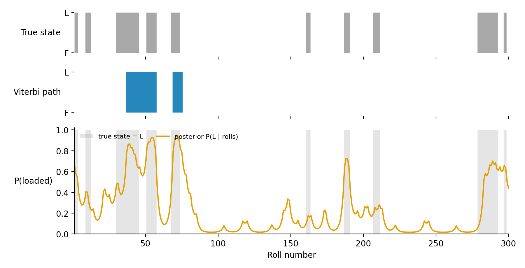
Figure 1.8: The occasionally dishonest casino. Top: the hidden state actually used for each of 300 rolls (grey = loaded). Middle: the Viterbi path decoded from the rolls alone. Bottom: the posterior probability \(P(\pi_i = L \mid x)\) from the forward–backward algorithm, with the true loaded segments shaded.

In this run of 300 rolls the loaded die was used for 21% of the rolls and 22% of all rolls were sixes. The Viterbi path assigns the correct state to 83% of the rolls, and thresholding the posterior at 0.5 gives 87%. The log-probability of the single best path is -550.7 nats, while the forward algorithm gives \(\log P(x) = -533.4\) nats for the sum over all paths.

Several general lessons can be read from the figure:

  • The Viterbi path is a “hard” answer that misses short loaded segments altogether. Switching into the loaded state costs \(\log 0.05\), which a few sixes cannot pay for.
  • The posterior is a “soft” answer. It rises in every loaded segment, even where Viterbi does not switch, and shows how uncertain the boundaries are.
  • The probability of the single best path is much smaller than the total probability of the sequence: many paths contribute. When the question is “does this sequence come from this model?”, the forward score is the right one to use, and this is what HMMER3 does.

The first rows of the dynamic-programming tables (natural logarithms) show the difference between taking the maximum (Viterbi, \(v\)) and the sum (forward, \(f\)) over predecessors. At the first roll both are identical; a six favours the loaded die. After that, the forward values are always at least as large as the Viterbi values.

\(t\) roll \(\log v_F(t)\) \(\log v_L(t)\) \(\log f_F(t)\) \(\log f_L(t)\) \(P(L\mid x)\)
1 6 -2.48 -1.39 -2.48 -1.39 0.67
2 3 -4.33 -3.79 -4.05 -3.78 0.58
3 6 -6.17 -4.59 -5.77 -4.53 0.55
4 5 -8.01 -7.00 -7.30 -6.93 0.39
5 3 -9.86 -9.41 -9.00 -9.30 0.31
6 2 -11.70 -11.82 -10.77 -11.63 0.28
7 3 -13.54 -14.22 -12.57 -13.92 0.28
8 4 -15.39 -16.63 -14.38 -16.13 0.32

1.6.5 Profile hidden Markov models

A profile HMM is an HMM whose architecture mirrors a multiple sequence alignment of a protein (or nucleic-acid) family (Krogh et al. 1994; Eddy 1998). Each consensus column of the alignment becomes a node with three states (Figure 1.9):

  • a match state \(M_k\), which emits a residue with column-specific probabilities \(e_{M_k}(a)\). This is the HMM equivalent of one column of a PSSM;
  • an insert state \(I_k\), which emits residues between columns \(k\) and \(k+1\), usually with background frequencies. Its self-transition \(I_k \to I_k\) allows insertions of any length;
  • a delete state \(D_k\), a silent state that emits nothing and lets the sequence skip column \(k\).
Figure 1.9: The core architecture of a profile HMM with four match states. Squares are match states (and the begin and end states), diamonds are insert states with self-loops, and circles are silent delete states. The transitions shown are those of HMMER’s Plan 7 architecture, which has no transitions between insert and delete states.

A path through the model from begin to end is an alignment of the sequence to the family. Matches use M states, insertions relative to the consensus use I states, and deletions use D states. Unlike a PSSM with fixed gap penalties, the transition probabilities differ between positions. A loop region where insertions are common in the family gets a high \(M_k \to I_k\) probability (a cheap gap), while a conserved core gets very expensive gaps. With log-odds scoring this is equivalent to position-specific affine gap penalties: the gap-open cost is \(\approx -\log a_{M_kI_k}\) (or \(-\log a_{M_kD_{k+1}}\)) and the extension cost \(\approx -\log a_{I_kI_k}\) (or \(-\log a_{D_kD_{k+1}}\)).

NoteProfiles, PSSMs, profile HMMs and pair HMMs are not the same

The terms are often used loosely, but they describe different models.

  • A PWM/PSSM gives a score for every residue at every position. A PWM for a motif has no gaps at all. The PSSM of PSI-BLAST is used with ordinary affine gap penalties that are the same at every position.
  • A Gribskov profile (and PROSITE’s generalised profiles) adds position-specific gap penalties, but the scores need not come from a probabilistic model.
  • A profile HMM models a family with explicit match, insert and delete states. Residue emissions and insertion and deletion behaviour are position-specific probabilities, and scores (including the forward score summed over all alignments) have a probabilistic interpretation.
  • A pair HMM models the alignment of two sequences, with one match and two gap states (Section 1.3). It is the probabilistic version of Gotoh’s algorithm and contains no family information.

Architecture: from Krogh’s model to Plan 7

The model of Krogh et al. (1994) had nine transitions per node, including transitions between insert and delete states. HMMER2 and HMMER3 use the simpler Plan 7 architecture, with seven transitions per node: \(M\to M\), \(M\to I\), \(M\to D\), \(I\to M\), \(I\to I\), \(D\to M\) and \(D\to D\). Removing \(I \leftrightarrow D\) transitions costs little, since an insertion directly followed by a deletion is rarely the best explanation of an alignment, and simplifies the algorithms.

Plan 7 also adds special states around the core model to control how a sequence may align to it:

  • N and C states emit unaligned flanking sequence before and after the match to the model (with background composition);
  • B and E are silent begin and end states of the core;
  • a J (“joining”) state allows the model to be used several times in one sequence. This is needed for proteins that contain several copies of the same domain.

Through the transitions out of B and into E, the same model can be used in different alignment modes. Global (with respect to the model) alignment requires the whole family model to be matched, from \(M_1\) to \(M_K\). Local alignment allows entry and exit at any match state, so that only a fragment of the model needs to be present. Local alignment with respect to both the model and the sequence corresponds to Smith–Waterman. Global with respect to the model but local with respect to the sequence is often called glocal. The N, C and J states make it multi-hit or uni-hit. HMMER3 searches use local (multi-hit) alignment by default, and the statistics for its forward scores are worked out for that mode.

Building a profile HMM from a multiple alignment

A profile HMM is usually estimated from a multiple sequence alignment (for example a Pfam seed alignment; Section 1.9) in a few steps. In HMMER this is done by hmmbuild.

  1. Choosing match columns. Columns in which a sufficient fraction of sequences have a residue (by default at least half, after weighting) become match states. The remaining columns are treated as insertions.
  2. Counting. With the columns assigned, the state path of every sequence is known, so emissions and transitions can be counted directly. No Baum–Welch is needed.
  3. Sequence weighting. Alignments are biased: they often contain many near-identical sequences from well-studied organisms. Weighting schemes down-weight redundant sequences, for example position-based weights that give more weight to sequences with rare residues in a column. HMMER3 also reduces the effective number of sequences so that the model has a target information content. This stops a model built from thousands of sequences from becoming too specific to detect distant members.
  4. Priors. Counts from a column with only a handful of sequences are poor estimates of the residue distribution of the whole family. They are combined with prior knowledge in the form of a Dirichlet mixture prior. Its components describe the typical kinds of alignment column (hydrophobic, aromatic, small, charged, conserved glycine, and so on). The posterior mean estimate of the emission probabilities is then \(e_{M_k}(a) = (c_{ka} + \alpha_a)/\sum_{a'}(c_{ka'} + \alpha_{a'})\) for a single Dirichlet component with parameters \(\alpha\). With a mixture, each component is weighted by how well it explains the observed counts. This is a principled replacement for the pseudocounts of PSI-BLAST.

Profile HMMs can also be trained from unaligned sequences with Baum–Welch, which simultaneously produces a multiple alignment (Krogh et al. 1994). This was demonstrated on globins and kinases. In practice, alignment programs (Section 1.6) followed by HMM estimation work better, because Baum–Welch easily gets stuck in poor local optima.

Scoring and statistics

To decide whether a sequence belongs to a family, its probability under the profile HMM is compared with its probability under a null model \(R\), usually a simple model that emits residues independently with background frequencies \(q_a\) (with a geometric length distribution). The score is the log-odds ratio, reported in bits (logarithm base 2):

\[ S = \log_2 \frac{P(x \mid \text{HMM})}{P(x \mid R)}. \]

With the Viterbi path instead of the sum, this reduces to a sum of position-specific log-odds scores, \(\log_2 \big(e_{M_k}(a)/q_a\big)\) for match emissions plus log transition probabilities, just like a PSSM with position-specific gap penalties. Because real sequences often have biased composition (low-complexity regions, transmembrane segments), HMMER also applies a second null model (“null2”) that corrects scores for composition bias.

A bit score must be converted into a measure of significance (see Section 1.4 for the general theory). Viterbi scores of local alignments of random sequences follow a Gumbel (extreme-value) distribution, as for BLAST. Eddy showed that a probabilistic local alignment model has a fixed slope parameter \(\lambda = \log 2\) when scores are in bits, both for Viterbi scores (Gumbel) and for forward scores (whose high-scoring tail is exponential) (Eddy 2008). Only the location parameter has to be estimated, which hmmbuild does with a short simulation. HMMER2 had needed a separate, slow calibration step (hmmcalibrate). This made it possible for HMMER3 to report E-values for forward scores. Summing over all alignments is more sensitive than using the single best one, because the alignment of a remote homologue is often uncertain. The E-value is, as in BLAST, the number of hits with at least this score expected by chance in a search of a database of this size.

HMMER and HMMER3

HMMER, written by Sean Eddy, is the standard implementation of profile HMMs. It is the engine behind Pfam, InterPro and many other family databases. HMMER1 appeared in the mid-1990s, and HMMER2 (1998) introduced Plan 7 and local alignment. Its main drawback was speed: a profile HMM search was 100–1000 times slower than BLAST, which limited it to searching the relatively small family databases. An independent profile HMM package, SAM (Sequence Alignment and Modeling system), was developed in parallel by the Santa Cruz group.

HMMER3 (Eddy 2011), a complete rewrite released in 2010, made profile HMM searches about as fast as BLAST without losing sensitivity. It uses a pipeline of increasingly expensive filters. Each target sequence must pass a score threshold, expressed as a P-value, to continue to the next stage:

  1. MSV filter (“multiple segment Viterbi”). This is an ungapped, local, multi-hit alignment of the model to the sequence. It finds one or more high-scoring ungapped segments, similar in spirit to BLAST’s ungapped extension. By default only about 2% of sequences (\(P < 0.02\)) pass.
  2. Viterbi filter. This is a full gapped Viterbi alignment, computed with reduced numerical precision. About 0.1% of sequences (\(P < 10^{-3}\)) pass.
  3. Forward filter. The full forward score in floating point, passed at \(P < 10^{-5}\).
  4. Domain definition and alignment. For the surviving sequences, forward–backward is used to compute posterior probabilities. From these HMMER identifies the individual domain hits and their boundaries, computes per-domain scores, and produces maximum expected accuracy alignments annotated with posterior probabilities.

The filters are fast because they are implemented with SIMD vector instructions. These process 16 one-byte scores (MSV) or 8 two-byte scores (Viterbi) in one instruction, using Farrar’s “striped” layout of the dynamic-programming matrix, originally developed for Smith–Waterman (Farrar 2006). Because the early filters only need to be accurate enough to reject non-homologues, they can use reduced precision. The expensive full computation is done only for the small fraction of sequences that might be true hits.

The HMMER package contains programs for different search directions:

  • hmmbuild builds a profile from an alignment;
  • hmmsearch searches a profile against a sequence database;
  • hmmscan searches a sequence against a profile database, for example annotating a protein with Pfam domains;
  • phmmer searches a single sequence against a sequence database, using a profile built from the sequence and a substitution matrix;
  • jackhmmer does iterative searches, like PSI-BLAST: each round builds a new profile HMM from the significant hits of the previous round. It was one of the programs used to build multiple alignments for AlphaFold2 (Jumper et al. 2021);
  • nhmmer and nhmmscan search DNA and RNA;
  • hmmalign aligns many sequences to a profile, which is how large alignments (such as Pfam full alignments) are built from a small seed.

Sequence and domain scores

HMMER output has two levels, which are often confused. The per-sequence score and E-value measure the evidence that a whole target sequence contains the family, summed over all its matches. The per-domain scores measure each individual match. The two can disagree. A protein with several weak copies of a repeat can be significant as a sequence although no single copy is; a multidomain protein can have one strong domain and a weak, doubtful second hit.

Each domain hit has two E-values. The independent E-value treats the domain as if it were the only hit and uses the whole database as the search space. The conditional E-value asks how significant the domain is given that the sequence has already been accepted as a member, and uses only the small number of sequences that passed. The conditional E-value is therefore much smaller and is meant for deciding whether additional, weaker domains in an accepted sequence are real; it is not a measure of database-wide significance. A report should say which statistic and which threshold were used.

Both HMMER and PSI-BLAST also separate a reporting threshold (which hits are shown) from an inclusion threshold (which hits count as members, and in iterative searches are used to build the next model). Changing the first only changes the output; changing the second changes the next profile, which is how profile drift begins.

Profile–profile comparison: the HH-suite

A profile HMM is more sensitive than a single sequence because it knows which positions are conserved and where gaps are likely. The logical next step is to represent both the query and the database entries as profile HMMs and align the two models. Johannes Söding’s HHsearch (Söding 2004) does this. It aligns two profile HMMs by a Viterbi-like dynamic programming over pairs of states. The score for aligning column \(i\) of the query with column \(j\) of the template is the log of the probability that the two match states emit the same residue (their co-emission probability), relative to the background:

\[ S_{aa}(q_i, t_j) = \log \sum_a \frac{q_i(a)\, t_j(a)}{f(a)}, \]

where \(q_i(a)\) and \(t_j(a)\) are the emission probabilities and \(f(a)\) the background frequencies. Optionally, a score for agreement between predicted and observed secondary structure is added. HHsearch, and the HHpred server built on it (Soding et al. 2005), became the most sensitive methods for detecting remote homologues of known structure, and HHpred-based servers performed among the best template-based modelling methods in several CASP experiments.

HHblits (Remmert et al. 2011) made the approach iterative and fast enough to search the whole sequence space. The database is first clustered (for example UniProt into clusters at about 20–30% identity: uniprot20, later Uniclust30 (Mirdita et al. 2016), and the metagenomic BFD). Each cluster is represented by a profile HMM built from its alignment. HHblits then searches this HMM database with a query HMM in a PSI-BLAST-like iterative way. Each round adds the sequences of the significant clusters to the query alignment. A two-stage prefilter, with fast ungapped and then gapped comparisons of discretised profile columns, reduces the tens of millions of database HMMs to a few thousand before the expensive HMM–HMM alignment. HHblits builds multiple alignments that are both deeper and more accurate than those from PSI-BLAST, in a fraction of the time. HH-suite3 (Steinegger et al. 2019) vectorised the HMM–HMM Viterbi and forward algorithms with SIMD instructions, much as HMMER3 did for sequence–profile comparison.

HH-suite tools are central to protein structure prediction (Chapter 9):

  • HHsearch against a database of PDB-derived profiles (PDB70) finds templates for homology modelling;
  • HHblits against Uniclust30 and BFD was used, together with jackhmmer, to construct the multiple sequence alignments that are the main input of AlphaFold2 (Jumper et al. 2021).

The deep, accurate alignments needed for coevolution analysis and deep learning are therefore a direct product of profile HMM methods. Today, much of this work is done with faster MMseqs2-based pipelines (Section 1.4).

How much do profiles gain?

Benchmarks on structurally classified proteins, where homology can be established from structure even when sequence similarity is undetectable, give a consistent picture. In a classic comparison, Park et al. (1998) showed that methods using multiple sequences (PSI-BLAST and the HMM program SAM-T98) detected about three times as many remote homologues as pairwise methods at the same error rate. Profile–profile methods add another substantial gain over sequence–profile methods (Söding 2004). The resulting ordering is

\[ \text{sequence–sequence} \;<\; \text{sequence–profile} \;<\; \text{profile–profile}. \]

The gain comes from more information on both sides, not from the HMM formalism alone. A PSSM built from a good alignment can come close to a profile HMM. The HMM’s advantages are position-specific gap probabilities, principled priors, the forward score and calibrated statistics.

Limitations

  • Independence of positions. A profile HMM assumes that columns evolve independently given the path. Correlations between positions, such as compensating mutations of residues in contact, are invisible to it. Models that capture them, such as Potts models and direct-coupling analysis, are the basis of coevolution-based contact prediction (Chapter 9). Protein language models (Section 1.10) learn such dependencies implicitly.
  • Simple length distributions. Self-loops give geometric distributions of insertion lengths, and a first-order Markov chain has no memory beyond the previous state. Gene finders use generalised HMMs with explicit length distributions for exons for this reason (Chapter 5).
  • Dependence on the alignment. A profile HMM is only as good as the multiple alignment it is built from. Misaligned regions or contaminating non-homologous sequences degrade it.
  • Profile drift. In iterative searches (jackhmmer, HHblits, PSI-BLAST), a single false positive included in one round can pull the profile towards an unrelated family. The search then reports many confident but wrong hits. Inclusion thresholds should therefore be conservative, and hits near the threshold should be checked (see the warning signs listed under PSI-BLAST above).
  • Local optima in training. Baum–Welch finds local maxima only, which is why profiles are usually estimated from fixed alignments.
TipQuestions to think about
  • Why is the forward score a better measure of homology than the Viterbi score for remote homologues, and why did it take until HMMER3 to use it in database searches?
  • How do the transition probabilities of a profile HMM relate to the gap penalties of Smith–Waterman? What can a profile HMM express that affine gap penalties cannot?
  • In what sense is a PSSM a special case of a profile HMM?
  • Why does an iterative search (PSI-BLAST, jackhmmer, HHblits) find more homologues than a single search, and what can go wrong?
  • Why is profile–profile comparison more sensitive than sequence–profile comparison?
NoteSources

Parts of this section are adapted from the Wikipedia articles Hidden Markov model, Viterbi algorithm, Forward algorithm, Forward–backward algorithm, Baum–Welch algorithm, HMMER and HH-suite (CC BY-SA 4.0, retrieved 2 October 2026). Parts of this section are adapted from Matteo Tadiello, Modern Bioinformatics: From Foundations to Frontiers, chapter “Sequence Databases, BLAST, and Profile HMMs” (CC BY 4.0), used with permission.

1.7 RNA homology search

The methods discussed so far work well for proteins, and for DNA that is very similar. Many genes, however, do not code for proteins. Their products are functional non-coding RNAs (ncRNAs). Examples are transfer and ribosomal RNAs, the RNA components of RNase P and the signal recognition particle, small nuclear and small nucleolar RNAs, microRNA precursors, riboswitches and many regulatory RNAs in bacteria and viruses. These molecules are among the oldest in the cell: ribosomal RNA is conserved across all of life and was the basis of the three-domain tree (Chapter 4). Yet ncRNA genes are notoriously hard to find by sequence similarity. This section explains why, and how the problem was largely overcome by extending profile HMMs (Section 1.6) to models that also describe RNA secondary structure.

1.7.1 Why RNA is different

The function of most ncRNAs depends on their structure, and the structure is formed largely by base pairing within the molecule. Complementary segments pair to form double-helical stems, connected by single-stranded hairpin loops, internal loops, bulges and multibranch loops. Besides the Watson–Crick pairs G–C and A–U, the G–U wobble pair is common. The set of base pairs is the molecule’s secondary structure. It is usually written in dot-bracket notation, where matching brackets mark paired bases and dots mark unpaired ones, for example ((((...)))) for a simple hairpin.

Three properties make RNA homology search harder than protein search:

  • In structured RNAs, structure is conserved better than sequence. In RNAs whose function depends on a conserved fold (tRNAs, rRNAs, RNase P RNA, riboswitches and many other structured ncRNAs), selection acts largely on the base pairs, not on the individual bases. A G–C pair can change to A–U, C–G or G–U with little effect on the structure. Such compensatory (or covarying) mutations change two positions of the sequence at once, while the structure stays the same. Two homologous RNAs can therefore share the same fold with very low sequence identity. A sequence-only method sees two mismatches where the evolutionary signal is in fact a conserved base pair. This is not a property of all RNA genes. Where function depends on sequence motifs, for example the seed region of a microRNA or a protein-binding site, sequence can be the more conserved feature, and some ncRNAs conserve neither (see Limitations below).
  • A small alphabet. With four nucleotides, a random position matches about a quarter of the time (1). Short ncRNAs of 70–300 nucleotides therefore give little statistical signal in a pairwise comparison.
  • Long-range dependencies. The two halves of a stem can be hundreds of nucleotides apart in the sequence. A profile HMM treats positions as independent given the state path, so it cannot represent the fact that position \(i\) must be complementary to position \(j\).

For close homologues, sequence-based tools work well enough: BLASTN, or profile HMMs for DNA such as nhmmer (Wheeler and Eddy 2013). For distant homologues, the structure has to be part of the model.

1.7.2 Predicting RNA secondary structure

Structure-aware search builds on algorithms for RNA folding, which are themselves dynamic programming (Section 1.3). The key simplification is that most base pairs in a secondary structure are nested: if \(i\) pairs with \(j\) and \(k\) pairs with \(l\), with \(i < k\), then either \(k\) and \(l\) both lie between \(i\) and \(j\), or both lie outside. Nested structures can be decomposed recursively, because the pair \((i, j)\) splits the sequence into an inside part and an outside part that do not interact. Structures that violate this rule are called pseudoknots. They occur in real RNAs, but they are usually left out of the models because they make the algorithms much more expensive.

  • Nussinov’s algorithm (Nussinov and Jacobson 1980) finds the structure with the maximum number of base pairs. The best structure of the subsequence \(x_i \ldots x_j\) is computed from the best structures of shorter subsequences: \(i\) is unpaired, \(j\) is unpaired, \(i\) pairs with \(j\), or the subsequence splits into two independent parts at some \(k\). Filling the table takes \(O(L^3)\) time and \(O(L^2)\) memory for a sequence of length \(L\).
  • Minimum free energy (MFE) folding (Zuker and Stiegler 1981) replaces “count the pairs” with a thermodynamic model. Most of the stability of a stem comes from stacking of adjacent base pairs, and loops cost energy depending on their type and size. The parameters (nearest-neighbour energies) are measured experimentally. The recursion has the same structure and the same \(O(L^3)\) complexity. This is the approach of programs such as mfold and the ViennaRNA package (RNAfold). A refinement computes the partition function, and from it the probability of every possible base pair, instead of a single optimal structure.

Single-sequence prediction is far from perfect. Many structures have similar energies, the energy parameters are approximate, and in the cell proteins and other RNAs influence the fold. Only a minority of predicted structures are correct in every pair, especially for long RNAs.

1.7.3 Comparative analysis: covariation

The most reliable evidence for an RNA structure comes from evolution. If an alignment of homologous RNAs shows that positions \(i\) and \(j\) always form a Watson–Crick or G–U pair, even though both positions vary, they are almost certainly paired. This comparative approach was used to determine the secondary structures of ribosomal RNAs and other large RNAs long before their crystal structures were known, and it proved remarkably accurate. Covariation can be measured with mutual information between alignment columns, or combined with folding energies to predict a consensus structure for the whole alignment, as in RNAalifold (Hofacker et al. 2002). It is the RNA counterpart of the coevolution analysis used for protein contact prediction (Chapter 9).

Covariation is only evidence if it exceeds what is expected from the phylogeny of the sequences alone. Closely related sequences share many substitutions simply by descent. R-scape (Rivas et al. 2016) tests whether the covariation of each proposed pair is statistically significant, given the phylogeny and the amount of variation in the alignment. Applied to published structures, it confirmed the pairs of well-established RNAs such as tRNA and rRNA. However, it found no significant support for the conserved structures proposed for several long non-coding RNAs. This is a useful reminder that a predicted structure, even in an alignment, is a hypothesis.

A harder problem is that structural alignment and structure prediction depend on each other. A correct structure requires a correct alignment, and for divergent RNAs a correct alignment requires knowing the structure. Sankoff (1985) gave a dynamic-programming algorithm that solves both simultaneously, folding and aligning two sequences at once. Its cost, \(O(L^6)\) time and \(O(L^4)\) memory for two sequences, makes it impractical in its full form. Tools such as LocARNA (Will et al. 2007) use restricted versions that work with base-pair probabilities and are fast enough to cluster thousands of ncRNA candidates into families.

1.7.4 From HMMs to stochastic context-free grammars

The step from profile HMMs to structure-aware models is easiest to see in the language of formal grammars. A grammar is a set of production rules that generate strings. In the Chomsky hierarchy, the simplest class, regular grammars, can only generate a string from left to right, with each step depending on the current state. HMMs are probabilistic regular grammars. Context-free grammars allow rules that emit symbols at both ends of a substring at once. For example,

\[ S \to \texttt{a}\,S\,\texttt{u} \;\mid\; \texttt{g}\,S\,\texttt{c} \;\mid\; \ldots \;\mid\; \varepsilon \]

generates nested complementary pairs, which is exactly the structure of an RNA stem. A stochastic context-free grammar (SCFG) attaches a probability to every rule. A parse of a sequence, the series of rule applications that generates it, then corresponds to a secondary structure, and its probability is the product of the rule probabilities.

The algorithms for SCFGs mirror those for HMMs (Section 1.6):

HMM SCFG Purpose
Viterbi CYK (Cocke–Younger–Kasami) most probable parse, i.e. structure or structural alignment
Forward Inside total probability of the sequence
Forward–backward Inside–outside posterior probabilities; training by EM

The price of modelling pairs is complexity. Where an HMM fills a table indexed by sequence position, an SCFG fills a table indexed by subsequences \((i, j)\). For a fixed grammar, the time is \(O(L^3)\) instead of \(O(L)\).

1.7.5 Covariance models

A covariance model (CM) is to an RNA family what a profile HMM is to a protein family. It is a profile SCFG built from a multiple alignment that is annotated with the family’s consensus secondary structure (Eddy and Durbin 1994). The consensus structure is converted into a tree of nodes. There are nodes for base pairs, for unpaired positions on the left or right, and bifurcation nodes where the structure branches into two stems, as in a multibranch loop. Each node is expanded into states, much like the match, insert and delete states of a profile HMM:

  • a pair state emits two nucleotides at once, with 16 probabilities for the 16 possible pairs. This is where covariation is captured: a family in which a position pair is G–C in some members and A–U in others gives high probability to both pairs, and low probability to mismatches such as G–A, even though each position on its own is variable;
  • states for single-stranded positions emit one nucleotide;
  • insert and delete states allow insertions and deletions relative to the consensus, with position-specific probabilities.

Parameters are estimated from the alignment with sequence weighting and Dirichlet priors, as for profile HMMs (Section 1.6). Sequences are scored by log-odds against a null model. Searching a genome means aligning the model to every window of the sequence. This scales roughly as the cube of the window length for every position of the genome, which made the first CM searches extremely slow.

1.7.6 Infernal

Infernal (“INFERence of RNA ALignment”), developed by Eric Nawrocki and Sean Eddy, is the standard implementation of covariance models. It plays the same role for RNA as HMMER does for proteins. The main problem was speed, and it was addressed in steps:

  • Banded dynamic programming. Query-dependent banding precomputes, for each state of the model, the range of subsequence lengths it can plausibly generate, and restricts the CYK and inside computations to these bands (Nawrocki et al. 2009). Bands can also be derived from a profile HMM alignment of the same sequence.
  • HMM filters. Infernal 1.1 (Nawrocki and Eddy 2013) adopted the filter pipeline of HMMER3 (Section 1.6). A profile HMM built from the same family first removes almost all of the genome using the fast MSV, Viterbi and forward filters. The full CM, with its much higher sensitivity, is only run on the remaining candidate regions. This made searches about 100 times faster than in Infernal 1.0.
  • Statistics. As in HMMER, scores are reported in bits with E-values calibrated on random sequences. Local alignment modes allow hits that cover only part of the model, including truncated hits at the ends of sequencing reads or contigs.

With these improvements, searching a whole bacterial genome for all known RNA families, or a CM against large sequence databases, became routine.

1.7.7 Rfam

Rfam is the database of RNA families, designed explicitly as the RNA counterpart of Pfam (Section 1.9). It was started in 2003 at the Sanger Institute, by Sam Griffiths-Jones, Alex Bateman, Sean Eddy and colleagues (Griffiths-Jones et al. 2003), and is now maintained at EMBL-EBI (Kalvari et al. 2020; Ontiveros-Palacios et al. 2024). Each family has:

  1. a curated seed alignment of representative sequences, annotated with the consensus secondary structure (in Stockholm format);
  2. a covariance model built from the seed with Infernal;
  3. a full alignment of all sequences in the database that score above the family’s manually chosen gathering threshold.

The same design as Pfam means that only the seed has to be curated, while the full alignments are regenerated automatically. Related families are grouped into clans. Like Pfam, Rfam links its family descriptions to Wikipedia, and many Wikipedia articles on RNA families were written in this collaboration. The database has grown from 25 families in the first release to several thousand today. Rfam 13 reorganised the database around complete reference genomes, and recent releases have added many families from viruses, metagenomes and microRNAs. Until release 12, the slowness of CMs meant that candidates were first found by BLAST, but Infernal 1.1 made this filter unnecessary.

Rfam is used to annotate ncRNA genes in newly sequenced genomes, much as Pfam and InterPro are used for proteins. Its main difficulty is the opposite of Pfam’s. Eukaryotic genomes contain many pseudogenes and repeats derived from ncRNAs, for example from tRNAs and small nuclear RNAs, which match the models well but are not functional genes. Separating these from the real genes requires additional evidence. Introns, which occur in some ncRNA genes, are also not described by the models.

1.7.8 Specialised tools: tRNAs

For the best-studied RNA families, specialised programs combine CMs with extra knowledge. tRNAscan-SE (Lowe and Eddy 1997; Chan et al. 2021) finds tRNA genes in genomes by first using fast filters, and then scoring the candidates with covariance models of the tRNA cloverleaf. The cloverleaf, with its acceptor stem, D arm, anticodon arm and T arm, is the classic example of a structure that is much better conserved than its sequence. tRNAscan-SE also identifies the anticodon and hence the amino acid specificity, and flags probable pseudogenes. It is used in essentially every genome annotation pipeline (Chapter 5).

1.7.9 Limitations

  • Pseudoknots and tertiary interactions cannot be represented by context-free models, so CMs ignore them. This loses some information, for example in riboswitches and RNase P RNA, where pseudoknots are conserved.
  • Cost. Even with filters, CM searches are much slower than profile HMM searches.
  • Dependence on the seed alignment. A CM is only as good as the structural alignment and consensus structure it is built from.
  • Not all ncRNAs are structured. Many long non-coding RNAs show little conservation of sequence or structure, and their function may depend on short sequence motifs or on the act of transcription itself. For them, structure-based homology search has little to offer, and homology can often only be inferred from conserved genomic position (synteny).

See also: further explanation in Section D.1.6; related Wikipedia articles in Section E.1.6.

NoteSources

Parts of this section are adapted from the Wikipedia articles Rfam, Probabilistic context-free grammar, Nucleic acid structure prediction and Non-coding RNA (CC BY-SA 4.0, retrieved 2 October 2026).

1.8 Whole-genome alignment and conservation

The methods earlier in this chapter align genes and proteins: sequences of a few hundred to a few thousand residues, whose homology is usually one-to-one along their length. Aligning whole genomes is a different problem, and its results, multiple genome alignments and the conservation scores computed from them, are among the most used tracks in genome browsers (Section 2.4).

1.8.1 Why genomes are not long genes

A genome alignment should identify, for every base, the homologous base (if any) in each of the other genomes. Several things make this harder than aligning two genes:

  • Rearrangements. Inversions, translocations, fusions and fissions break the collinearity of genomes (Section 6.5). A single global alignment, as computed by Needleman–Wunsch, cannot represent a block that has moved or changed orientation.
  • Duplications and losses. A region may have one copy in one genome and several in another, through segmental or whole-genome duplication. The alignment must then decide which copy is the orthologue, or allow one base to align to several.
  • Repeats. Transposable elements and other repeats make up about half of mammalian genomes. They create huge numbers of short, spurious matches, so repeats are usually soft-masked (written in lower case) and used only to extend alignments, not to start them.
  • Size and divergence. Mammalian genomes are billions of bases long, and most of their sequence is neutrally evolving, so between distant species only a small part can be aligned with confidence.

Whole-genome alignment is therefore done in stages: find local matches, chain them into collinear blocks, and decide which blocks represent orthology.

1.8.2 Pairwise alignment: BLASTZ/LASTZ, chains and nets

BLASTZ was developed to align the human and mouse genomes (Schwartz et al. 2002). It follows the seed-and-extend scheme of BLAST (Section 1.4), but with spaced seeds (by default 12 matching positions in a window of 19, with one transition allowed), which are more sensitive for diverged non-coding DNA than contiguous words. The best seed is not fixed: it depends on the length and similarity of the matches that are sought, so seed patterns and word sizes are search parameters to be tuned rather than constants (Gotea 2003). The seeds are followed by gapped extension and a second, more sensitive search between the anchors that were found. Its successor LASTZ is used in the same way.

The local alignments are then organised in two steps, introduced at UCSC (Kent et al. 2003):

  • A chain is an ordered series of gapless blocks that are in the same order and orientation in both genomes. Gaps are allowed in both sequences between blocks, which is how insertions, deletions and unalignable sequence appear. Chains are found by dynamic programming over the local alignments, much like the chaining of seeds in minimap2.
  • A net is a hierarchical selection of chains in which each base of the reference genome is covered at most once. The best chain is placed first, and gaps in it are filled with the best chains that fit there. Nets therefore distinguish the orthologous, collinear alignment from alignments to paralogous copies, and they show inversions and other rearrangements as nested chains.

Chains are also the basis of liftOver, the tool that converts coordinates between assemblies of the same genome (Section 2.4).

1.8.3 Multiple genome alignment

Pairwise alignments to one genome can be combined into a multiple alignment. MULTIZ, part of the threaded blockset aligner (Blanchette et al. 2004), progressively merges pairwise alignments that all share a reference genome, following a phylogenetic tree. The UCSC multiple alignments of vertebrates and mammals are built this way. Such alignments are reference-based: they only contain sequence that aligns to the reference (for example human), and sequence absent from the reference is lost.

Reference-free methods treat all genomes symmetrically. In Ensembl, Enredo builds a graph of collinear segments from anchors in all genomes, allowing for duplications and rearrangements, and Pecan aligns each segment with a consistency-based method in the spirit of T-Coffee (Section 1.6) (Paten et al. 2008). Progressive Cactus (Armstrong et al. 2020) represents the alignment as a cactus graph, in which rearrangements and duplications are natural, and aligns genomes progressively along a guide tree, reconstructing an ancestral genome at each internal node. Because each new genome only has to be aligned to its nearest ancestors, the method scales to hundreds of genomes. It was used to build the Zoonomia alignment of about 240 mammal species (Genereux et al. 2020; Christmas et al. 2023) and alignments of hundreds of bird genomes.

1.8.4 Evaluating genome alignments

There is no ground truth for real genomes, so genome aligners are hard to evaluate. The Alignathon competition (Earl et al. 2014) compared aligners on genomes simulated with a known evolutionary history, including rearrangements and duplications, where precision and recall of aligned base pairs can be computed, and on real fly genomes, where only indirect measures are possible. Methods differed substantially, especially for distant genomes, and no method was best on all measures. The lesson matches that for protein alignment (Section 1.11): a genome alignment is an estimate, and downstream results, such as which bases are conserved, inherit its errors.

1.8.5 Conservation scores

Given a multiple genome alignment and a phylogenetic tree with a neutral model of substitution, usually estimated from sites assumed to evolve without constraint, such as fourfold degenerate sites or ancient repeats, each column can be asked: did it change less than expected? Purifying selection removes mutations at functional positions, so a deficit of substitutions is evidence of function, whether or not the sequence codes for protein. Three scores are widely used:

  • phastCons (Siepel et al. 2005) uses a two-state phylo-HMM (Section 1.6): a hidden Markov model along the genome whose states emit alignment columns according to a phylogenetic model. In the conserved state all branch lengths are scaled down by a factor \(\rho < 1\). The posterior probability of the conserved state is reported for each base, and runs of high probability are called conserved elements. Because neighbouring bases share a state, phastCons finds elements rather than single positions.
  • phyloP (Pollard et al. 2009) tests each base (or element) separately for a departure from the neutral rate, and reports \(-\log_{10}\) \(p\)-values: positive for conservation (slower than neutral) and negative for acceleration (faster than neutral). It can also test one lineage, for example the human branch, which is how human accelerated regions, conserved in other mammals but rapidly changed in humans, were found (Pollard et al. 2006).
  • GERP (Cooper et al. 2005) measures constraint as rejected substitutions: the number of substitutions expected at a column under neutrality minus the number estimated to have occurred. A score of 4 means that four substitutions that would have happened have been removed by selection. GERP++ (Davydov et al. 2010) calls constrained elements from these scores.

Conservation scores are used to find functional non-coding elements, such as enhancers and non-coding RNAs, and to estimate how much of the genome is under constraint (Section 6.9). They are also among the most informative features for interpreting variants: a variant at a strongly constrained base is more likely to be harmful, and base-level constraint from the Zoonomia alignment helps to prioritise non-coding variants in rare disease and association studies (Sullivan et al. 2023). Scores such as CADD include phyloP and GERP among their features (Section 10.6), and variant calling itself is described in Section 5.4.

Conservation scores also have important limitations:

  • They depend on the alignment. Misaligned paralogues, assembly errors and missing data in some species look like substitutions or conservation. Repeats are often poorly aligned and therefore under-scored.
  • They need enough evolution. Single-base resolution requires a large total branch length in the tree. A handful of primates cannot show that a single base is constrained; hundreds of mammals can. Alignments of distant species, on the other hand, contain only the most conserved elements.
  • Function can be lineage-specific. Elements that are new or turn over quickly, such as many transcription factor binding sites, are not conserved across the tree although they are functional in one lineage. Lack of conservation is therefore not evidence of lack of function.
  • Not all deviation is selection. Mutation-rate variation and GC-biased gene conversion can make a region look conserved or accelerated, as discussed for some human accelerated regions.

A conserved base is evidence that some function has been maintained by selection over the depth of the tree used. It does not say what the function is, or whether it is the same in humans.

See also: further explanation in Section D.1.10; related Wikipedia articles in Section E.1.10.

NoteSources

Written for this book from the primary literature cited in the text.

1.9 Databases and domains

So far we have mostly treated a protein as one sequence to be aligned from end to end, or at least as one region of local similarity. Real proteins are often built from several independent parts, domains, that have their own evolutionary histories. A protein of 800 residues may share one domain with a kinase, another with a transcription factor, and a third with nothing in the databases at all. Understanding domains is therefore essential for interpreting search results. It also explains why the most widely used annotation resources, Pfam and InterPro, are organised around domains and families rather than whole proteins. This section covers what a domain is, how domain families are built and searched (Pfam, Pfam-N and InterPro), and gives a first look at the structural classifications (SCOP, CATH, ECOD and TED) that are discussed further in Chapter 2 and Chapter 9.

1.9.1 What is a protein domain?

History of the concept

The idea of the domain grew out of the first protein crystal structures. In 1973 Donald Wetlaufer surveyed the structures then available, including hen lysozyme, papain and fragments of immunoglobulins produced by limited proteolysis. He noted that many proteins consist of separate, compact globular regions that are connected only by a few strands of polypeptide chain (Wetlaufer 1973). He proposed that such regions are stable units of protein structure that can fold autonomously, and suggested that folding of a large protein proceeds by nucleation within these regions. The immunoglobulins were a particularly clear case. Proteolysis cut the antibody into fragments that kept their structure and binding activity, and the sequence of each chain could be seen to consist of repeats of about 110 residues, each forming one compact “immunoglobulin domain”.

As more structures were determined, the term came to be used in three overlapping senses:

  • Structural domain: a compact, globular sub-structure with more contacts within itself than with the rest of the protein, and usually with its own hydrophobic core.
  • Folding domain: a unit that can fold, and remain stable, on its own when expressed or cut out of its parent protein.
  • Evolutionary (and functional) domain: a unit that recurs in different proteins and different combinations. It has been moved around as one piece by gene duplication, fusion and recombination during evolution, and often carries a recognisable function, such as binding a ligand or catalysing a reaction.

In most cases these definitions agree: a compact structural unit found in many different proteins usually also folds on its own. But they need not agree, and different databases make different choices. This is one reason why domain boundaries and domain counts differ between resources.

Size and structure of domains

Domains are typically 50–250 residues long. Individual structural domains range from about 36 residues (in E-selectin) to almost 700 (in lipoxygenase), but about 90% are shorter than 200 residues, and the average is around 100 residues. Very small domains, below about 40 residues, are usually stabilised by metal ions or disulphide bridges; zinc fingers are the classic example. Domains longer than about 300 residues often turn out to contain more than one hydrophobic core and can be split further.

Each domain is built from secondary structure elements packed around a core. Domains are traditionally grouped into four classes by their secondary-structure content: all-α, all-β, α/β (mostly parallel β-sheets with β-α-β units, as in the TIM barrel or the Rossmann fold) and α+β (helices and mostly antiparallel strands in separate regions). These classes form the top level of both SCOP and CATH (below).

A domain need not be a single continuous stretch of sequence. When one domain has been inserted into a loop of another during evolution, the host domain is made up of two or more segments of the chain. Pyruvate kinase is the textbook example: its TIM-barrel domain is interrupted by an inserted β-barrel domain. About a quarter of structural domains are discontinuous in this way. A practical consequence is that a domain cannot always be represented by a single start and end position in the sequence, which complicates both sequence-based domain databases and automatic domain assignment.

Long-range interactions also matter in the other direction. Some proteins form oligomers by domain swapping, where a secondary-structure element or a whole domain of one chain replaces the equivalent part of a neighbouring chain. And in many multidomain proteins the domains are connected by flexible, often intrinsically disordered linkers, so their relative orientation varies. This is one reason why structure-based domain assignment, and structure prediction (Chapter 9), is usually more reliable for individual domains than for whole chains.

1.9.2 Multidomain proteins and domain architectures

Multidomain proteins are common, especially in eukaryotes. Estimates depend on the definitions and databases used, but roughly 40% of prokaryotic proteins and 65–80% of eukaryotic proteins are multidomain proteins, and the fraction is highest in multicellular animals (Apic et al. 2001). The linear order of domains along the chain, from N- to C-terminus, is called the protein’s domain architecture.

Figure 1.10 shows three classic examples:

  • Src tyrosine kinase has an N-terminal unique region followed by an SH3 domain, which binds proline-rich peptides; an SH2 domain, which binds phosphotyrosine; and a C-terminal kinase domain. The same SH2 and SH3 domains occur, in other combinations, in hundreds of other signalling proteins.
  • Tissue plasminogen activator consists of a fibronectin type-I (“finger”) module, an EGF-like module, two kringle domains and a trypsin-like serine protease domain. The extracellular proteins of blood clotting, fibrinolysis and complement are built from a small set of such modules, combined in many different ways. They were among the first examples of domain shuffling, the reuse of domains through exon shuffling and recombination.
  • The purine-biosynthesis enzymes GARs, AIRs and GARt are three separate proteins in bacteria. In yeast, GARs and AIRs are fused into one chain while GARt is separate, and in vertebrates all three are fused into a single trifunctional polypeptide. The same activities are present in all three, but the way they are packaged into chains differs.
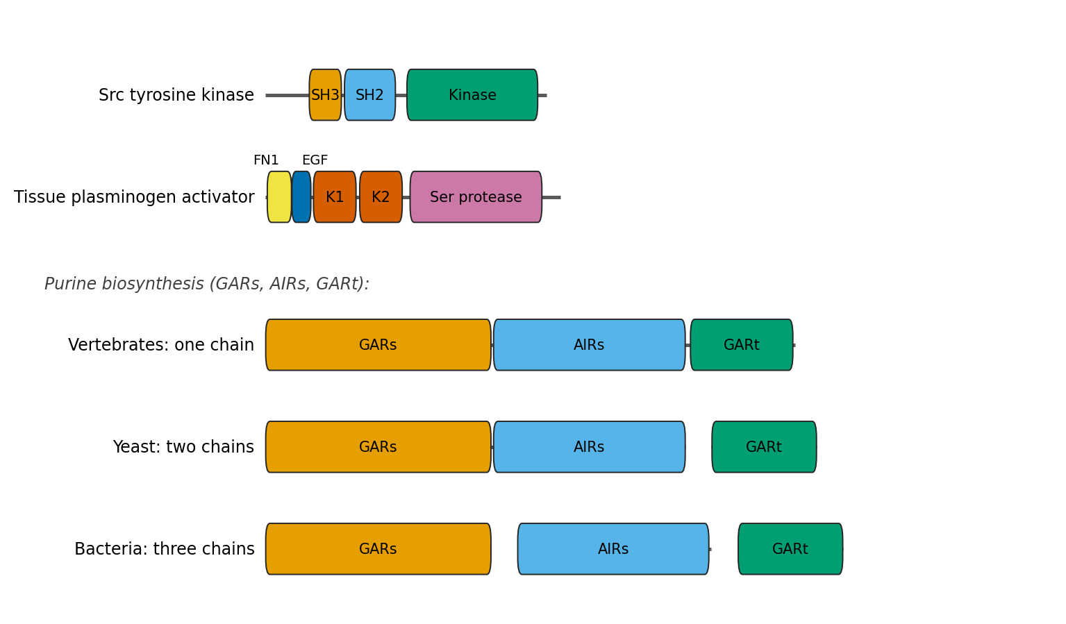
Figure 1.10: Schematic domain architectures (approximately to scale). Top: Src kinase and tissue plasminogen activator, two multidomain proteins built from widely reused domains (K1, K2: kringle domains; FN1: fibronectin type-I module). Bottom: the purine-biosynthesis enzymes GARs, AIRs and GARt are separate chains in bacteria, partly fused in yeast and fully fused in vertebrates.

The last example illustrates a general pattern. Many domains that form parts of multidomain proteins in eukaryotes exist as separate proteins in prokaryotes, which suggests that multidomain proteins have often arisen by gene fusion of previously independent genes. The opposite process, gene fission, also occurs. Because fused proteins usually function together, the observation that two proteins are fused in another genome is used to predict functional links (“Rosetta stone” proteins, Chapter 10).

How domain architectures evolve

Domain architectures change through a limited set of genetic mechanisms: duplication of a whole gene or part of it, fusion and fission, insertion of one domain into another, exon shuffling (in eukaryotes, where introns make recombination between domains easier), and transposition, including horizontal transfer between species. Several broad patterns have been found by comparing architectures across genomes:

  • Combinations are limited. Although thousands of domain families are known, only a small fraction of all possible pairs of domains is ever observed together, and most domains combine with only one or two partners. A few promiscuous domains, such as SH3, SH2, PH and the immunoglobulin domain, combine with very many others (Basu et al. 2008). Domain combinations also tend to keep their N-to-C order (Apic et al. 2001).
  • Most changes happen at the ends. When architectures of related proteins are compared, most differences are the gain or loss of single domains at the N- or C-terminus, rather than insertions in the middle (Björklund et al. 2005).
  • Tandem repeats are common. The simplest architecture is one domain repeated many times. Titin, a muscle protein of about 30,000 residues, contains more than a hundred immunoglobulin and fibronectin type-III domains. In some repeats, as in the two β-barrels of the trypsin-like serine proteases, the copies have diverged so far that their common origin is only visible in the structure.
  • Assembly mirrors evolution. For protein complexes, the order in which subunits assemble often reflects the order in which they were added during evolution (Levy et al. 2008).

These patterns, and how domain rearrangements relate to gene duplication and to the evolution of new functions, are discussed further in Chapter 3.

Why domains matter for sequence searching

Domains have direct consequences for the search methods in this chapter:

  • Hits are local. A significant hit between two multidomain proteins usually means that one region is homologous, not the whole chain. Local alignment (Section 1.3) will report the shared domain, but the rest of the two proteins may be unrelated.
  • Annotation transfer can go wrong. If the query shares only an SH2 domain with a kinase, transferring the annotation “tyrosine kinase” is a mistake. Many errors in sequence databases have arisen in exactly this way and have then propagated as other proteins were annotated from the erroneous entries (Chapter 10).
  • Homology is not transitive across domains. If protein A matches B through domain 1, and B matches C through domain 2, then A and C are not shown to be related at all. Iterative methods such as PSI-BLAST, and sequence clustering by single linkage, can “walk” from one family to another through multidomain proteins in this way. This is a common source of profile corruption (Section 1.6).
  • Search per domain. For these reasons, sequences are often annotated by searching them against libraries of domain models, such as Pfam, instead of (or as well as) against whole sequences. Boundaries found in that way can then be used to cut a protein into domains before further analysis.
  • Low-complexity and repeat regions (compositionally biased segments, coiled coils, transmembrane helices, short repeats) can produce high-scoring but non-homologous matches. They are often masked before searching, and are handled specially in domain databases.

1.9.3 Pfam

Pfam is the most widely used database of protein domains and families. It contains a curated multiple sequence alignment and a profile hidden Markov model (Section 1.6) for each family, and it is used to annotate the protein content of essentially every newly sequenced genome.

History

Pfam was started in 1995 by Erik Sonnhammer, Sean Eddy and Richard Durbin at the Sanger Centre in Cambridge, and was first described in 1997 (Sonnhammer et al. 1997). A major motivation was the annotation of the first animal genome, that of the nematode Caenorhabditis elegans. The project was also inspired by Cyrus Chothia’s argument (Chothia 1992) that most proteins belong to a limited number of families, perhaps around a thousand. If so, a manageable collection of family models could annotate a large fraction of all proteins. The estimate turned out to be too low: Pfam release 37.0 (June 2024) contains almost 22,000 families. But the main idea, that a library of family models gives broad and sensitive coverage, has been borne out. Already around release 29, about three quarters of all sequences in UniProtKB had at least one Pfam match.

Pfam was originally a consortium with sites in the UK, the USA and Sweden (Erik Sonnhammer, who now works at Stockholm University and SciLifeLab). Between 2012 and 2014 it moved to the European Bioinformatics Institute (EMBL-EBI), and since about 2022 it has been part of InterPro, through whose website it is now accessed (Mistry et al. 2020; Paysan-Lafosse et al. 2022).

How a Pfam family is built

What made Pfam different from earlier collections was its use of two alignments for each family, and of profile HMMs to connect them (Sonnhammer et al. 1997):

  1. Seed alignment. A curator assembles a small, high-quality multiple alignment of representative members of the family. Sequences are taken from a non-redundant database of reference proteomes (pfamseq) and the alignment is checked by hand. Candidate families come mainly from proteins of known structure in the PDB, and from proteins in complete proteomes that have no Pfam match yet.
  2. Profile HMM. A profile HMM is built from the seed alignment with HMMER (hmmbuild) (Eddy 1998).
  3. Search. The HMM is searched against the full sequence database (hmmsearch). With HMMER3 (Eddy 2011), this became roughly a hundred times faster than before, which made frequent updates possible.
  4. Full alignment. All sequences scoring above the family’s threshold are aligned to the HMM. This gives the full alignment, which can contain millions of sequences.

The key advantage of this design is that only the small seed alignment has to be maintained by hand. When the sequence database grows, the full alignment is regenerated automatically by searching again with the HMM.

Thresholds: GA, TC and NC

Each Pfam family has a manually set gathering threshold (GA), a bit score above which a match is accepted as a member of the family. HMMER scores are given both for the whole sequence and for each individual domain match, and the GA has a value for both. The curator chooses the threshold to include as many true members as possible while excluding false positives. Pfam also records two derived values:

  • the trusted cutoff (TC), the lowest score of any sequence included in the family;
  • the noise cutoff (NC), the highest score of any sequence that was not included.

The gap between NC and TC indicates how cleanly the family is separated from the background. False positives are recognised mainly as overlaps: if a region matches two different families that are not known to be related, at least one of the matches is probably wrong. Thresholds are re-checked at each release to prevent such overlaps. In practice, using the curated thresholds (--cut_ga in HMMER) is usually more reliable than using a fixed E-value cutoff for all families.

Entry types, clans and domains of unknown function

Pfam entries are classified as families, domains, repeats or motifs. “Family” is the default and just means that the members are related. “Domain” means an autonomous structural unit that can occur in different protein contexts. “Repeat” denotes units that are not stable on their own and only form a structure as tandem copies. “Motif” denotes short units, usually outside globular domains.

As families grew and more structures were solved, it became clear that many Pfam families are themselves distantly related. Since 2005 such families have been grouped into clans (Finn et al. 2006): sets of families that are believed to share a common evolutionary origin, based on structural similarity, functional similarity, and HMM–HMM comparison (Section 1.6). Pfam curators also use the ECOD structural classification (below) to identify clan relationships. A clan corresponds roughly to a superfamily in the structural classifications, but the two are defined on different units and need not coincide (see the table at the end of this section). Families in the same clan are not allowed to overlap in the same sequence region, so the best-scoring member family is reported.

A substantial part of Pfam consists of domains of unknown function (DUFs): families that are clearly conserved across species but whose function has not been determined. They are named DUF followed by a number and are renamed when a function is found. Since around 2010 more than a fifth of all Pfam families have been DUFs, and their share has grown as new genomes are sequenced. Many DUFs are good targets for experimental work.

Pfam-A and Pfam-B

The curated families described above form Pfam-A. Since they did not cover all proteins, Pfam also provided Pfam-B, a large set of automatically generated families from sequence clustering. Pfam-B families were of lower quality, but could give a hint when no Pfam-A family matched. Pfam-B was discontinued with release 28.0 and later reintroduced (release 33.1), now generated with MMseqs2 clustering (Section 1.4).

Community curation through Wikipedia

Writing functional descriptions for thousands of families is more than a small curation team can do. From release 26.0, Pfam (together with its sister database Rfam for RNA families) therefore linked family descriptions to Wikipedia articles. Existing articles were connected to the corresponding families, and the community was invited to write new ones. Edits are reviewed by Pfam curators before they appear on the Pfam pages. Many Wikipedia articles on protein domains therefore originate from, and are maintained together with, Pfam.

1.9.4 Pfam-N: deep learning for domain annotation

Profile HMMs are sensitive, but they still miss many sequences that do belong to a family, especially in poorly studied lineages and metagenomes. In 2022, Maxwell Bileschi, Lucy Colwell and colleagues at Google Research showed that deep neural networks can be trained to classify protein sequences into Pfam families directly (Bileschi et al. 2022). Their model, ProtCNN, is a convolutional neural network (Chapter 12) trained on Pfam seed alignments. It takes a protein domain sequence as input and outputs the probability that it belongs to each Pfam family. An ensemble of such networks (ProtENN) was then combined with HMMER.

Two features of this work are important. First, the networks were evaluated on a split of the data in which test sequences had low sequence identity to the training sequences. This tests the ability to detect remote homologues rather than near-duplicates, a point that applies to all machine-learning methods in bioinformatics (Chapter 12). On such a split, the deep models made fewer classification errors than profile HMMs, and the combination of the two was better than either. Second, the models were used to annotate UniProt sequences that had no Pfam match. This added several million new domain annotations and raised Pfam’s coverage of UniProtKB by roughly a tenth. These predictions are distributed as Pfam-N (“N” for neural).

Pfam-N annotations are kept separate from the HMM-based ones, because they come with different evidence and different error properties. Curators also use them to extend the seed alignments of the standard families. This is part of a broader shift: recent Pfam releases also use AlphaFold-predicted structures to check and correct family boundaries, and to identify new families and clan relationships (Paysan-Lafosse et al. 2024).

1.9.5 InterPro

Pfam is one of several “signature” databases, each modelling families, domains or sites in its own way: regular expressions (PROSITE patterns), position-specific scoring matrices (CDD, PROSITE profiles), fingerprints (PRINTS) and profile HMMs (Pfam, SMART, TIGRFAMs/NCBIfam, PANTHER, CATH-Gene3D, SUPERFAMILY, PIRSF, HAMAP). InterPro, at EMBL-EBI, integrates these member databases into a single resource (Paysan-Lafosse et al. 2022). Signatures from different databases that describe the same family, domain or site are merged into one InterPro entry, with a common name, description and Gene Ontology terms. Entries are linked in parent–child relationships (for example, a family and its subfamilies) and classified by type (family, domain, repeat, site, homologous superfamily). InterPro precomputes matches for all of UniProtKB; more than 80% of its sequences have at least one match (Blum et al. 2020; Paysan-Lafosse et al. 2022). The InterProScan software lets users run all member databases on their own sequences. InterPro is now the standard starting point for annotating a new protein, and the databases are discussed further in Chapter 2.

1.9.6 Structural classification of domains

Because structure among homologues tends to be conserved much longer than sequence, many evolutionary relationships between domains can only be seen at the structural level. Several databases therefore classify domains of known three-dimensional structure. They are only introduced here; structure itself is the topic of Chapter 9.

SCOP

The Structural Classification of Proteins (SCOP) was created in 1994 by Alexey Murzin, Steven Brenner, Tim Hubbard and Cyrus Chothia at the MRC Laboratory of Molecular Biology and the Centre for Protein Engineering in Cambridge (Murzin et al. 1995). SCOP is largely manual: the classification was based on expert inspection of structures, supported by sequence comparison. Its unit is the structural domain, and its main levels are:

  • Class: the overall secondary-structure content (all-α, all-β, α/β, α+β and some special classes).
  • Fold: domains with the same major secondary structures in the same arrangement and with the same topological connections. A shared fold does not by itself imply common ancestry; similar folds can arise by convergence because only a limited number of arrangements are physically favourable.
  • Superfamily: domains in the same fold that have low sequence identity but whose structural and functional features together indicate a probable common ancestor.
  • Family: domains with clear sequence similarity (typically more than 30% identity), or lower identity combined with very similar structure and function. These are closely related homologues.

The human trypsin domain, for example, is classified as all-β class, trypsin-like serine protease fold, trypsin-like serine protease superfamily, eukaryotic protease family. The original SCOP was updated until version 1.75 (2009). It is continued as SCOPe at Berkeley (Fox et al. 2013), which adds new structures in a largely automated but compatible way, and as SCOP2 from the Cambridge group (Andreeva et al. 2019), which replaces the strict tree with a more flexible network of relationships.

CATH

CATH was created in the mid-1990s by Christine Orengo, Janet Thornton and colleagues at University College London, and is still developed by the Orengo group (Sillitoe et al. 2020). Protein chains from the PDB are “chopped” into domains by a combination of algorithms and curation, and each domain is classified in four main levels, which give the database its name:

  • Class (C): secondary-structure content (mainly α, mainly β, α–β, few secondary structures).
  • Architecture (A): the overall arrangement of secondary structures in space, regardless of how they are connected (e.g. sandwich, barrel, three-layer sandwich).
  • Topology (T): the fold, i.e. the arrangement and connectivity of the secondary structures.
  • Homologous superfamily (H): domains with good evidence of a common ancestor.

Below the H level, CATH groups domains into sequence clusters and functional families (FunFams). Compared with SCOP, CATH relies more on automatic structure comparison, has an explicit architecture level, and does not use the α+β class. Through its sister resource Gene3D, CATH superfamilies are represented by HMMs that are used to assign domains to sequences without known structure, and Gene3D is one of the InterPro member databases.

ECOD

ECOD (Evolutionary Classification of Protein Domains), from Nick Grishin’s group at UT Southwestern, puts evolutionary relationships first (Cheng et al. 2014). Its levels are architecture (A), possible homology (X), homology (H), topology (T) and family (F). The X level is the most distinctive: it groups domains for which homology is plausible but not established, instead of forcing a yes-or-no decision. Higher levels are defined by evidence of common ancestry rather than by shape alone, so domains with different topologies can still be placed in the same homology group if other evidence supports it. ECOD is updated weekly from the PDB, and its families map closely onto Pfam families, which is why Pfam uses it when defining clans.

TED: domains across the AlphaFold Database

Until recently, structural classifications covered only the roughly 200,000 experimentally determined structures in the PDB. The AlphaFold Protein Structure Database (Varadi et al. 2021) changed this by providing predicted structures for more than 200 million UniProt sequences. The Encyclopedia of Domains (TED) (Lau et al. 2024), from the Orengo and Jones groups at UCL together with others, used these models to segment and classify domains at the scale of the whole protein universe.

Chopping that many structures by hand is impossible. TED therefore combined three deep-learning domain-segmentation methods (Chainsaw, Merizo and UniDoc) and accepted domain boundaries on which they agreed. Applied to about 188 million unique AlphaFold models, this identified nearly 365 million domains. Using structure comparison (including Foldseek, Section 1.4), about 194 million of these could be assigned to known CATH superfamilies, and a further 46 million matched known CATH topologies. The rest have structures not previously classified in CATH, and include many candidate new folds. TED shows both how much of protein space is covered by known folds, and how much remains unexplored.

Structure classifications and homology

The structural hierarchies connect directly to the definition of homology in 1. Homology means common ancestry; it is not a degree of similarity. Placing two domains in the same superfamily (SCOP, CATH) or homology group (ECOD) is a statement that there is enough evidence (structural similarity together with shared functional details, unusual structural features or weak sequence similarity) to conclude that they are homologous, even when their sequence identity is too low for sequence methods to detect it. Placing them only in the same fold or topology says that they have similar architectures, but leaves open whether this reflects common ancestry or convergence. The TIM barrel is the standard example: it is found in many enzyme families catalysing unrelated reactions, and it is still debated whether all TIM barrels share a common ancestor. The structure databases, in other words, help us infer homology, but similarity of structure, like similarity of sequence, is evidence for homology and not the same thing.

The same words have different meanings in different databases, which is a frequent source of confusion. Table 1.1 compares them.

Table 1.1: Domain-classification terms in different databases.
Term Database Meaning
Domain SCOP, CATH, ECOD, TED A structural unit, cut out of a structure (experimental or predicted).
Pfam, InterPro A region matched by a sequence model; in Pfam also one entry type, for units that occur in different protein contexts.
Family SCOP Domains with clear sequence similarity (often above 30% identity) or very similar structure and function.
Pfam The default entry type: any set of related sequences modelled by one HMM, which may be a domain, part of a domain or a whole protein.
ECOD (F), CATH (FunFam) ECOD: sequence-based families, close to Pfam families. CATH FunFams: functionally coherent subgroups within a superfamily.
Superfamily / homology group SCOP, CATH (H), ECOD (H) Domains judged to share a common ancestor from structural, functional and weak sequence evidence.
Possible homology ECOD (X) Homology plausible but not established.
Clan Pfam Sequence families believed to share a common ancestor (from structure, function and HMM–HMM comparison). Roughly a superfamily, but built from Pfam families, so its boundaries and membership can differ.
Fold / topology SCOP (fold), CATH (T) Same secondary structures in the same arrangement and connectivity; no claim of common ancestry. In ECOD, T is instead a level below the homology group.

See also: further explanation in Section D.1.7; related Wikipedia articles in Section E.1.7.

NoteSources

Parts of this section are adapted from the Wikipedia articles Protein domain, Pfam, Structural Classification of Proteins database, CATH database and InterPro (CC BY-SA 4.0, retrieved 2 October 2026).

1.10 Protein language models

Every method in the previous sections compares sequences residue by residue, with scores that come from explicit models of evolution: substitution matrices, profiles, HMMs. Since about 2019 a different idea has spread from natural-language processing into biology. A large neural network is trained to predict amino acids from their sequence context on hundreds of millions of natural protein sequences, without any labels. To do this well, the network learns, implicitly, which substitutions are tolerated at which positions, which residues tend to be in contact and which sequence patterns belong to which families. Its internal representations, the embeddings, can then be used for prediction tasks and, more recently, to search for homologues. These networks are called protein language models (PLMs). This section describes where they come from, what they learn, and how they are being used for sequence searching and the detection of remote evolutionary relationships. The machine learning background is covered in Chapter 12.

1.10.1 From words to residues

The distributional hypothesis

In linguistics, the idea that “a word is characterised by the company it keeps” goes back to John Rupert Firth in 1957. This distributional hypothesis says that words occurring in similar contexts tend to have similar meanings. In natural-language processing it led to word embeddings: each word is represented by a real-valued vector, learned so that words that appear in similar contexts end up close together in the vector space. Early approaches reduced the dimension of word co-occurrence matrices, for example by latent semantic analysis in the late 1980s. From about 2000, neural probabilistic language models learned distributed representations directly, and word2vec (2013) made this cheap enough to train on very large text collections.

A protein sequence can be read in the same way. The tokens are the twenty amino acids (plus a few special symbols), a protein is a “sentence”, and the “corpus” is a sequence database such as UniProt or UniRef (Chapter 2). The analogy is useful but imperfect. The protein alphabet is tiny compared with a natural vocabulary, so a single residue carries little meaning on its own. What a residue “means” depends almost entirely on its context: the same leucine may be buried in a helix in one protein and exposed in a loop in another. A useful protein model therefore needs contextual embeddings, where the representation of a residue depends on the whole sequence around it. The evolutionary interpretation of the distributional hypothesis is also clear. The sequences in the corpus are the survivors of natural selection, so the patterns of co-occurring residues reflect structural and functional constraints. These are the same constraints that give rise to conserved columns in a multiple alignment (Section 1.6) and to correlated mutations between residues in contact (Chapter 9).

Language modelling objectives

A language model assigns probabilities to sequences. Two training objectives dominate.

  • Autoregressive (causal) language modelling. The model predicts each residue from the residues before it, so that the probability of a sequence \(x = x_1 \dots x_L\) factorises as \[ p(x) = \prod_{i=1}^{L} p(x_i \mid x_1, \dots, x_{i-1}). \] This is the objective of the GPT family in natural language. Such models can also generate new sequences, one residue at a time.
  • Masked language modelling. This is the objective popularised by BERT (2018). A random subset \(M\) of positions (typically about 15%) is hidden, by replacing the residues with a mask token, and the model is trained to recover them from the remaining, unmasked context on both sides. The loss for one sequence is \[ \mathcal{L} = -\sum_{i \in M} \log p\left(x_i \mid x_{\setminus M}\right), \] where \(x_{\setminus M}\) denotes the sequence with the masked positions hidden. The model never sees labels such as structure or function. This is self-supervised learning: the training signal is the sequence itself.

How well a model has learned is often summarised by its perplexity, the exponential of the average negative log-likelihood per residue. A model that knows nothing has a perplexity of about 20 (a uniform guess over the amino acids). Lower values mean the model predicts the hidden residues better.
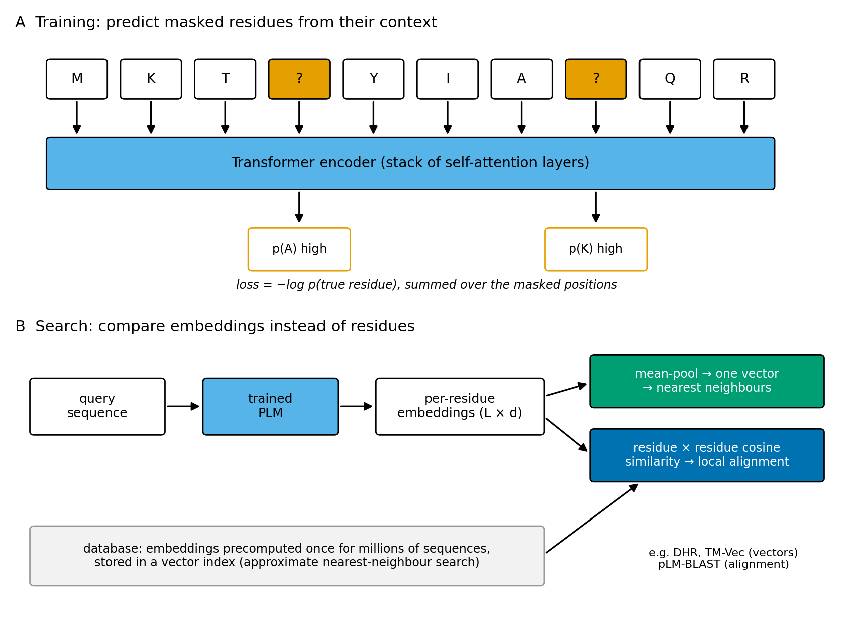
Figure 1.11: Protein language models. (A) In masked language modelling, some residues are hidden and the network is trained to predict them from the rest of the sequence. (B) After training, the per-residue embeddings can be compared directly, either as one pooled vector per protein (nearest-neighbour search) or residue by residue (alignment of embeddings).

Recurrent networks and transformers

The first protein language models used recurrent neural networks, in particular long short-term memory (LSTM) networks. These read the sequence one position at a time and carry information forward in a hidden state. They are hard to parallelise, and information from distant positions is easily lost.

The transformer (Vaswani et al. 2017) removed the recurrence. Each token is first converted into a vector by an embedding layer. Positional information is added, because attention by itself ignores order. Each layer then updates every token’s vector by self-attention, a weighted combination of all the other tokens in the sequence. For a sequence represented as a matrix of token vectors, three learned linear maps give queries \(Q\), keys \(K\) and values \(V\), and attention is computed as \[ \mathrm{Attention}(Q, K, V) = \mathrm{softmax}\!\left(\frac{Q K^{\top}}{\sqrt{d_k}}\right) V, \] where \(d_k\) is the dimension of the keys. The matrix \(\mathrm{softmax}(QK^{\top}/\sqrt{d_k})\) is an \(L \times L\) table that says how much each position “looks at” every other position. Several such attention heads run in parallel in each layer, and many layers are stacked.

Two properties make transformers attractive for proteins. All positions are processed in parallel, so very large models can be trained on GPUs. And any position can interact directly with any other, which suits proteins, where residues far apart in sequence are often close in space. The price is that the cost of attention grows quadratically with sequence length. Most protein models are therefore trained on sequences cropped to around 1,000 residues.

1.10.2 A short history of protein language models

Early embeddings

Representing biological sequences with learned vectors predates the current models. In 2015 Asgari and Mofrad adapted word2vec to proteins (“ProtVec”) (Asgari and Mofrad 2015), treating overlapping amino-acid 3-mers as words. These context-free embeddings carried some information about family membership and physico-chemical properties. However, they ignore the order and context of the 3-mers and were soon superseded.

Recurrent models: UniRep and SeqVec (2019)

The first models that learned contextual representations from large sequence collections appeared in 2019. UniRep (Alley et al. 2019) was a multiplicative LSTM trained autoregressively, to predict the next amino acid, on about 24 million UniRef50 sequences. Averaging its hidden states over the sequence gave a fixed-length vector per protein. Simple regression models on top of this vector could predict stability and the effects of mutations, and the authors used it to guide protein engineering. SeqVec (Heinzinger et al. 2019) adapted ELMo, a bidirectional LSTM language model from natural-language processing, to UniRef50. Per-residue embeddings from SeqVec, used as input to small supervised networks, predicted secondary structure and disorder. Per-protein embeddings predicted subcellular localisation and membrane association. These predictions approached, but did not reach, methods that used evolutionary information from multiple sequence alignments. They were, however, much faster, because no database search was needed.

Around the same time, the TAPE benchmark (Rao and colleagues, 2019) compared several architectures on a common set of tasks, such as secondary structure, contacts, remote homology, fluorescence and stability. It showed that self-supervised pre-training helps on almost all of them. On the structural tasks, however, it still did not reach features derived from alignments.

Transformers at scale: ESM-1b and ProtTrans (2020–2021)

The next step was to train much larger transformers on much more data. ESM-1b (Rives et al. 2021), from the group of Alexander Rives at Facebook AI Research, was a 33-layer transformer with about 650 million parameters. It was trained with masked language modelling on UniRef50, which the authors drew from a collection of about 250 million sequences. The paper analysed what the model had learned without supervision:

  • the embeddings of the amino acids themselves clustered by physico-chemical properties (hydrophobic, aromatic, charged and so on);
  • per-protein embeddings separated orthologous groups and reflected phylogenetic relationships;
  • per-residue embeddings contained information on secondary structure and on which residues are in contact;
  • these signals improved as the model’s perplexity decreased.

Shortly afterwards, Rao and colleagues showed that the attention maps of such models predict residue–residue contacts directly (Rao et al. 2020). A simple logistic regression on the attention weights recovered contacts with accuracy comparable to coevolution methods based on a full multiple alignment. The model had, in effect, learned something similar to the coupling analysis of Chapter 9, but from single sequences.

ProtTrans (Elnaggar et al. 2022), from the group of Burkhard Rost in Munich, trained several transformer architectures from natural-language processing on UniRef and on the metagenomic Big Fantastic Database (BFD), with billions of sequences in total. The models included ProtBERT, an encoder trained by masked language modelling, and ProtT5, an encoder–decoder model. The encoder of ProtT5-XL became one of the most widely used sources of embeddings. Using only its embeddings, without alignments, the authors predicted secondary structure about as well as the best alignment-based methods of the time. They also predicted localisation and membrane association well. A review by Bepler and Berger (2021) summarises this period and discusses how evolution, structure and function are encoded in the learned representations.

Structure from a language model: ESM-2 and ESMFold (2022–2023)

ESM-2 (Lin et al. 2023) scaled the masked-language-model approach to a series of models from 8 million to 15 billion parameters, trained on UniRef. As the models grew, their perplexity fell and the contact information in their attention maps increased. ESMFold attaches a structure module, similar to that of AlphaFold2 (Jumper et al. 2021), to the ESM-2 language model. It predicts atomic structures from a single sequence, without searching for homologues or building an alignment. ESMFold is less accurate than AlphaFold2 on average, especially for proteins with few homologues. Because it skips the alignment step, however, it is roughly an order of magnitude faster. The authors used it to predict more than 600 million structures from metagenomic sequences (the ESM Metagenomic Atlas). An important observation was that ESMFold’s accuracy is closely related to the language model’s perplexity on the sequence. The model works well when it “understands” a protein, which in practice usually means that related sequences were well represented in its training data.

Generative and multimodal models (2024–)

The most recent models go beyond sequence. ESM3 (Hayes et al. 2025) is a generative masked language model that reasons over three tracks at once: sequence, structure and function. Structure is encoded as discrete tokens, and function as keyword annotations. Any combination can be given as a prompt and the rest generated. The largest version has about 98 billion parameters. As a demonstration, the authors generated a functional green fluorescent protein, esmGFP, that is only distantly related to known fluorescent proteins. This illustrates a broader trend: language models are increasingly used to design sequences (Chapter 9), not just to analyse them. Other models in this family include autoregressive models trained to generate protein families, and “bilingual” models that translate between amino-acid sequence and structural alphabets.

1.10.3 What do embeddings capture?

It is worth being precise about what a PLM provides. For a protein of length \(L\), the last layer of the network (or a chosen intermediate layer) gives one vector of dimension \(d\) per residue, an \(L \times d\) matrix. Typically \(d\) is between about 1,000 and 5,000. This per-residue embedding is used for tasks that need a prediction for each residue, such as secondary structure, disorder, binding sites, transmembrane segments or signal peptides (Chapter 10). Averaging the vectors over all positions (mean pooling) gives a per-protein embedding of fixed size \(d\). This is used for tasks about the whole protein, such as localisation, enzyme class or family membership, and for fast comparison of proteins.

“The embedding of a protein” is therefore not a uniquely defined object. It depends on the model, on the layer it is taken from (intermediate layers are sometimes better than the last), and, for a per-protein vector, on the pooling: mean pooling, the vector of a special start token, maximum pooling, or a learned (attention-based) pooling. Long sequences may also be cropped or split into chunks, which changes the result. Pooling discards the order of the residues, so two proteins with similar composition and local environments but different domain order can get similar per-protein vectors. Embeddings are therefore only comparable when they were computed with the same model, layer and pooling.

Several lines of evidence show what these representations contain:

  • Structure. Secondary structure and solvent accessibility can be read from per-residue embeddings with small supervised models. Contacts can be read from attention maps, and full 3D structures can be built from the representations (ESMFold).
  • Function. Per-protein embeddings cluster by enzyme class, Gene Ontology terms and subcellular localisation. Simple nearest-neighbour annotation in embedding space (“embedding-based annotation transfer”) often works where sequence similarity is too low for BLAST.
  • Evolution. The likelihood a masked model assigns to a mutation correlates with the measured fitness effect of that mutation in deep mutational scanning experiments. This makes PLMs useful as unsupervised predictors of variant effects (Meier et al. 2021) (Chapter 10).
  • Family membership. Proteins from the same family or superfamily are often close in embedding space, even when sequence identity is in the twilight zone (1). This is an empirical ability to recover family and structural relationships, not a direct inference of ancestry. Closeness in embedding space can also reflect shared structure class, composition or function, so on its own it is not evidence of common ancestry in the sense of a significant alignment score.

A common interpretation is that a large PLM acts as a compressed multiple sequence alignment. During training it sees many members of each family. The weights then store the conservation and covariation patterns that a profile or coevolution model would extract from an explicit alignment, and the model “retrieves” this information when it sees a new member of the family. This view explains both the strengths and the main weakness of PLMs. They are good for proteins from large, well-sampled families. For orphan proteins, or families with few sequences in the training data, they know little more than what is in the query itself.

1.10.4 Using language models to search for homologues

Classic homology search compares residues with a substitution matrix (Section 1.3) or a profile (Section 1.6). Embeddings offer two new possibilities. First, two proteins can be compared through their embeddings instead of their residues. Second, because an embedding summarises a sequence in context, it may carry information about structure and family that the raw sequence only reveals through an alignment with many homologues. Several types of methods have appeared since 2021.

Predicting structural similarity from sequence

Because structure among homologues tends to be conserved longer than sequence, structural similarity is the most sensitive sign of remote homology (1). It normally requires structures, which led to Foldseek and its 3Di alphabet (van Kempen et al. 2023) (Section 1.4). TM-Vec (Hamamsy et al. 2023) instead trains a network on top of PLM embeddings to predict the TM-score between two proteins, a measure of structural similarity (Chapter 9), directly from their sequences. The network is trained on pairs of proteins with known structures, so that the cosine similarity of the two output vectors approximates their TM-score. A database is again indexed once, and a query returns the proteins predicted to have similar structures, even when sequence identity is very low. The companion method DeepBLAST predicts a structural alignment between the two sequences.

A related idea uses language models to predict the 3Di structural alphabet directly from sequence (for example ProstT5 (Heinzinger et al. 2024), a “bilingual” model derived from ProtT5). This allows Foldseek-style structural search for proteins without any predicted structure.

Aligning embeddings

Pooling an \(L \times d\) embedding into a single vector throws away the positional information needed for an alignment. An alternative keeps the per-residue embeddings and uses them in place of a substitution matrix. pLM-BLAST (Kaminski et al. 2023) computes the cosine similarity between every residue embedding of the query and every residue embedding of the target. This gives an \(L_1 \times L_2\) similarity matrix specific to that pair of sequences, which is then used in a Smith–Waterman-like local alignment (Section 1.3). Since the embedding of a residue depends on its context, the matrix effectively contains a position-specific substitution score for each pair, much like a profile–profile comparison, but obtained from two single sequences. On benchmarks of distant homology, pLM-BLAST detects relationships that BLAST misses and performs comparably to HMM–HMM comparison with HHsearch (Section 1.6), without building alignments for either sequence. Methods of this type also show where in two sequences the similarity lies, which pooled embeddings cannot.

Combined pipelines

Practical tools combine these ideas to balance speed and sensitivity, in the same way that BLAST and MMseqs2 combine a fast prefilter with a slower alignment step (Section 1.4). PLMSearch (Liu et al. 2024) first filters candidate pairs, using predicted family membership and embedding similarity. It then scores the remaining pairs with a model that predicts structural similarity from ESM embeddings, and finally aligns the hits with an embedding-based alignment method. The authors reported sensitivity for remote homologues similar to structure-based search, at a speed close to that of MMseqs2.

Deep learning for family annotation

Closely related to search is the assignment of sequences to known families. ProtCNN (Bileschi et al. 2022) is a deep convolutional network trained to classify sequence domains into Pfam families. It is not a transformer language model, but it rests on the same idea of learned sequence representations. Combined with profile HMMs, it was used to create Pfam-N, which added millions of new family assignments to UniProt sequences that the Pfam HMMs had missed. This is discussed in Section 1.9.

1.10.5 How good are they?

Remote-homology methods are usually evaluated on benchmarks derived from structural classifications such as SCOP or CATH (Section 1.9). Pairs in the same superfamily but in different families count as true remote homologues, and pairs in different folds count as non-homologues. Methods are compared by how many true pairs they rank above the first false one, or by the area under ROC-type curves. On such benchmarks, embedding-based methods are often more sensitive than BLAST and MMseqs2 in the twilight zone, and in several studies match or exceed HMMER and HHblits (Eddy 2011; Remmert et al. 2011). They usually remain below full structural comparison when structures are available.

These results have to be read carefully, for reasons that are directly relevant to the exam’s emphasis on understanding the limitations of methods.

  • Leakage between training and test data. A language model is trained on essentially all known sequences, including the test proteins and their relatives. A supervised model on top of it may be trained on pairs from the same families as the benchmark. Unless training and test sets are separated by family or superfamily, not just by sequence identity, reported performance is likely to be optimistic (the same issue as in any supervised learning in biology; Section 12.2).
  • No well-founded statistics. The great strength of BLAST, HMMER and MMseqs2 is that their scores come with E-values derived from a model of random alignments (Section 1.4). A cosine similarity or a predicted TM-score has no such theory behind it. Thresholds are set empirically, and the false-positive rate on a new database is hard to predict. Some methods calibrate their scores against shuffled or unrelated sequences, but this is less mature than for classic tools.
  • Bias towards well-sampled families. As discussed above, PLMs work best where training data are rich. Orphan proteins, rapidly evolving families, viral proteins and de novo designed proteins are often poorly represented, and these are precisely the cases where a sensitive remote-homology method is needed most.
  • Cost. Searching an index is fast, but computing embeddings for hundreds of millions of sequences with a large model needs GPUs and a lot of storage. Each per-residue embedding is thousands of numbers per residue. The indexes must also be rebuilt when the model changes.
  • Interpretability. An HMMER hit can be explained by the alignment and the profile columns that match. An embedding similarity is much harder to explain, although methods that align embeddings (pLM-BLAST) recover some of this.

1.10.6 Outlook

PLMs have not replaced classic sequence searching. They have added a new layer to it. Profile HMMs and fast \(k\)-mer-based tools remain the standard for routine annotation, because they are well understood, their statistics are reliable, and they run on ordinary computers. Language models are most useful at the edge of what these methods can detect: in the twilight zone, for building alignments quickly, for annotating metagenomic sequences at scale, and as cheap stand-ins for structural comparison. The classic and new approaches are also merging. Profile and alignment information is used to train language models, and language models are used to produce substitution scores, structural alphabets and alignments that feed into dynamic programming. It is therefore important to understand both: what the older methods assume, and why a model trained only to fill in missing amino acids ends up with representations from which evolutionary, structural and functional relationships can be recovered.

See also: further explanation in Section D.1.8; related Wikipedia articles in Section E.1.8.

NoteSources

The background on word embeddings, the distributional hypothesis and the transformer architecture is adapted from the Wikipedia articles Word embedding, Transformer (deep learning) and Large language model (CC BY-SA 4.0, retrieved 2 October 2026). There is no Wikipedia article on protein language models. The rest of the section is based on the papers cited.

1.11 Benchmarking search methods

Each method in this chapter claims to be more sensitive, faster or more accurate than its predecessors. At the exam you should be able to say how such claims are tested, and what can go wrong. The central problem is that we need to know the right answer: which pairs of sequences are truly homologous and which are not. That knowledge must come from somewhere other than the method being tested.

1.11.1 Where does the truth come from?

The most widely used source of truth is a structural classification (Section 1.9). Because structure among homologues tends to be conserved much longer than sequence, two domains classified in the same SCOP or CATH superfamily are taken to be homologous, even if they have no detectable sequence similarity. Domains in different folds are taken to be unrelated. Pairs in the same fold but different superfamilies are ambiguous (they may be distant homologues or analogues) and are usually excluded. These labels are an operational gold standard: a convenient, independent definition of right and wrong answers, not a complete record of evolutionary history. Early benchmarks used curated sequence superfamilies instead (Pearson 1995). The SCOP-based benchmark of Brenner et al. (1998) became the template for later work. It showed that pairwise methods found only a small fraction of the homologous pairs with less than about 30% identity, and that well-computed E-values were reliable indicators of significance. Park et al. (1998) used the same approach to show that profile methods find about three times as many remote homologues, and Lindahl and Elofsson (2000) measured performance separately at the family, superfamily and fold levels. Their results showed that methods which work well for close relationships can fail almost completely at the fold level, so a single overall number can hide large differences.

Other reference sets are used for other tasks: structural superpositions for multiple alignments (BAliBASE, Thompson et al. (1999)), and blind prediction experiments for structure and function (CASP and CAFA; Chapter 9 and Chapter 10).

1.11.2 What is measured?

A search method returns a ranked list of hits with scores or E-values. Performance is described by how true and false hits are ordered in that list.

  • ROC curves. The receiver operating characteristic curve plots the number (or fraction) of true positives against false positives as the score threshold is lowered. The area under the curve (AUC) summarises it. In a database search almost all pairs are negatives, and only the top of the list is ever examined. The ROC\(_n\) score is therefore often used. It is the area under the curve up to the \(n\)th false positive, for example ROC\(_1\) or ROC\(_{50}\) (Gribskov and Robinson 1996).
  • Coverage versus errors per query. Brenner et al. (1998) plotted the fraction of true relationships found (coverage) against the number of false positives per query. This shows directly how many homologues are found at an acceptable error rate.
  • Sensitivity up to the first false positive, per query, averaged over all queries, is a common simple summary (used, for example, in the Foldseek and MMseqs2 papers; Section 1.4).
  • E-value calibration. If E-values are correct, a search should produce on average \(E\) false positives with E-value at most \(E\) per query. Plotting the observed number of false positives against the reported E-value tests whether a method’s statistics can be trusted. This is as important as sensitivity, because users choose thresholds based on E-values.
  • Speed, in queries per hour or as a speed-up over BLAST, is always reported with a sensitivity measure. A faster method is only an improvement if it loses little sensitivity.

1.11.3 Pitfalls

Benchmarks are easy to design badly, and many published comparisons contradict each other for that reason.

  • Circularity. If the reference set was built with one of the methods being compared, that method has an advantage. For example, Pfam families are defined by HMMER searches, so HMMER will look good on a benchmark based on Pfam membership.
  • Bias towards large families. If every pair counts equally, a few very large superfamilies dominate the result. Results are usually weighted per query or per family, and redundant sequences are removed (for example, keeping only domains below 40% identity to each other).
  • “False” positives that are true. Disagreement with a database classification is not automatically a biological false positive. Structural classifications are incomplete: relationships between superfamilies are still being discovered, and two superfamilies may later be merged or placed in the same ECOD homology group. Domain boundaries differ between SCOP, CATH and ECOD, and the schemes use different criteria for homology (Table 1.1). A hit counted as false may therefore be a real homologue classified in another superfamily, or a match to another domain in a multidomain protein. Ambiguous pairs should be excluded rather than counted as errors, and apparently false hits with very good scores are worth inspecting: some of them are discoveries.
  • Leakage in machine-learning methods. A method that has been trained on sequences from the same families as the test set can appear to detect remote homologues while in fact recognising families it has seen. Training and test sets must be separated by superfamily or fold, not only by sequence identity. This is particularly important for deep-learning and language-model methods (Section 1.10), whose pre-training data may include the benchmark proteins themselves. Homology between training and test (or benchmark) sets is one of the most common reasons for inflated performance in bioinformatics, and it affects structure, function and interaction predictors as much as search methods; see Section 12.2.
  • Tuning on the test set. Parameters chosen to maximise performance on a benchmark will overestimate how well a method works on new data. Independent test sets, or blind assessments such as CASP, avoid this.

When you read a claim that a new method “outperforms” existing ones, it is worth asking: what was the reference, how were true and false pairs defined, which measure was used, and could the method have seen the test data?

See also: further explanation in Section D.1.9; related Wikipedia articles in Section E.1.9.

NoteSources

Parts of this section are adapted from the Wikipedia article Receiver operating characteristic (CC BY-SA 4.0, retrieved 2 October 2026).

1.12 Key concepts

A checklist for revision. You should be able to explain each point, including the algorithm or argument behind it, and its limitations.

  • Homology: definition as common ancestry (qualitative, not a percentage); orthologues, paralogues (in-/out-paralogues), xenologues, ohnologues; analogy and convergence; why significant similarity implies homology but not the reverse; the twilight and midnight zones; why proteins are compared rather than DNA
  • Dynamic programming: principle of optimality; Needleman–Wunsch and Smith–Waterman recursions and traceback; semi-global, overlap and banded alignment; linear, affine and convex gap penalties; Gotoh’s three-matrix algorithm; time and space complexity, Hirschberg/Myers–Miller linear space
  • Substitution matrices: log-odds scores, target and background frequencies, relative entropy; how PAM and BLOSUM are derived and how their numbering differs; choosing a matrix
  • Heuristic search: FASTA (\(k\)-tuples, diagonals, banded optimisation); BLAST (neighbourhood words, threshold \(T\), X-drop, two-hit method, gapped extension); low-complexity filtering; the BLAST family and translated searches; DIAMOND, MMseqs2 and Linclust; Foldseek and the 3Di alphabet
  • Statistics: why local scores follow a Gumbel distribution; Karlin–Altschul \(E = Kmn\,e^{-\lambda S}\); bit scores, E- and P-values; effective lengths, gapped and composition-based statistics; why E-values depend on database size while the score does not; per-query E-values versus multiple testing over many queries; query and target coverage
  • From hit to annotation: checking the query (gene model, fragments, low complexity); identity with its denominator, coverage of both sequences and domain architecture; why the best (or reciprocal best) hit is not necessarily the orthologue; escalating to profiles, structure or embeddings without lowering the evidence standard; annotation statements that match the evidence; recording database release, program version and parameters
  • Exact matching: suffix trees and arrays; the Burrows–Wheeler transform, LF mapping, FM-index and backward search; why they suit read mapping
  • Multiple alignment: no single correct objective (SP, consistency, probabilistic and structure-aware surrogates); sum-of-pairs score and NP-hardness; progressive alignment and “once a gap, always a gap”; ClustalW, Clustal Omega, T-Coffee (consistency), MUSCLE and MAFFT (iterative refinement); benchmarks; alignment uncertainty, MUSCLE5 ensembles and trimming as a modelling choice
  • Motifs and profiles: consensus, PROSITE patterns, PWMs with pseudocounts, information content and logos; Gibbs sampling and MEME; Gribskov profiles; sequence weighting and priors; computing a PSSM with background-weighted pseudocounts; PSI-BLAST and profile corruption (how to recognise and limit it); PSSM vs. profile HMM vs. pair HMM
  • Hidden Markov models: states, transitions, emissions; Viterbi, forward, backward, posterior decoding and Baum–Welch; profile HMM architecture (match/insert/delete, Plan 7), local and glocal modes; HMMER3 filter pipeline and forward-score E-values; per-sequence vs. per-domain scores, independent vs. conditional E-values, reporting vs. inclusion thresholds; HHsearch/HHblits (HMM–HMM comparison); sequence–sequence < sequence–profile < profile–profile
  • Domains: structural, folding and evolutionary definitions; multidomain proteins and architectures; why domains complicate annotation transfer; Pfam (seed/full alignments, gathering thresholds, clans), Pfam-N, InterPro; SCOP, CATH, ECOD and TED, and fold vs. superfamily; database-specific meanings of family, superfamily and clan
  • RNA homology search: why structured RNA homologues often conserve structure better than sequence; compensatory mutations and covariation; Nussinov and Zuker folding algorithms; SCFGs and their relation to HMMs (CYK, inside–outside); covariance models, Infernal and its HMM filters; Rfam; limitations (pseudoknots, unstructured ncRNAs)
  • Whole-genome alignment and conservation: why genomes are not aligned like genes (rearrangements, duplications, repeats, soft-masking); BLASTZ/LASTZ with spaced seeds; chains and nets; reference-based (MULTIZ) vs. reference-free (Enredo–Pecan, Progressive Cactus) multiple genome alignment and the Zoonomia alignment; Alignathon and the lack of ground truth; neutral models; phastCons (phylo-HMM), phyloP (conservation and acceleration, human accelerated regions) and GERP (rejected substitutions); use for non-coding elements and variant interpretation; caveats (alignment errors, branch length needed, lineage-specific function, biased gene conversion)
  • Alignment-free comparison: \(k\)-mer statistics; MinHash and the Mash distance; ANI and Kraken; when alignment-free methods work and when they fail
  • Protein language models: masked and autoregressive objectives; transformers and attention; UniRep, SeqVec, ESM, ProtTrans, ESMFold, ESM3; per-residue and per-protein embeddings and pooling; embedding search, TM-Vec, pLM-BLAST, PLMSearch; limitations (leakage, lack of statistics, bias towards well-sampled families)
  • Benchmarking: structural classifications as an operational ground truth (and why disagreement is not always an error); ROC, ROC\(_n\), coverage vs. errors per query, E-value calibration; circularity, family-size bias and train–test leakage

1.14 Background reading (open access)

Descriptions of Wikipedia articles are taken from the introductions of the articles (CC BY-SA 4.0).

1.15 Student recommendations

Recommended by students preparing for the exam: papers, reviews, online lectures, tutorials and short explanations. To suggest something, use the suggestion form (SU login).

No recommendations yet.

1.16 Review problems

These problems are adapted from Matteo Tadiello, Modern Bioinformatics: From Foundations to Frontiers (CC BY 4.0), used with permission. For a longer treatment of this topic, see the chapters “Sequence Alignment and Search Foundations” and “Sequence Databases, BLAST, and Profile HMMs” of that book. In the HTML version, click a box to show the extensions, solution outline and common errors.

1.16.1 Derive global and local alignment

Derive the dynamic-programming recurrences for global and local pairwise sequence alignment. Explain which biological questions each formulation answers, and why neither recurrence gives a uniquely true evolutionary alignment.

Extensions:

  • Give the optimal-substructure argument from the three possible final columns of an alignment.
  • Compare initialisation, termination and traceback for global, local and semi-global alignment.
  • Derive the time and memory complexity for sequences of lengths \(n\) and \(m\).
  • How would you test whether the result for a protein pair with uncertain terminal homology depends on the alignment mode?

Solution outline:

  1. Define \(F_{ij}\) as the optimal score of the prefixes \(A_{1:i}\) and \(B_{1:j}\); the final column must be a residue pair or a gap in one of the two sequences.
  2. Write the recurrence with a diagonal, a vertical and a horizontal move, using a substitution score and a linear gap cost.
  3. For global alignment, penalise leading gaps and trace back from \(F_{nm}\). For local alignment, add zero to the maximum, initialise the first row and column to zero, start the traceback at the highest cell and stop at a zero.
  4. State \(O(nm)\) time and \(O(nm)\) memory for the traceback matrix; distinguish computing the score alone in linear memory from reconstructing the alignment (Hirschberg, Myers–Miller).
  5. Use global alignment for sequences expected to correspond over most of their lengths, local alignment for a shared domain or a fragment, and semi-global alignment when terminal gaps should be free.
  6. Conclude that the optimum depends on the substitution scores, the gap model, the boundary conditions and any masking.

Common errors:

  • Describing the optimum under one scoring system as the biological truth.
  • Changing only the traceback, without the zero and the boundary conditions of local alignment.
  • Aligning proteins with different domain architectures globally without considering alternatives.

Connections: Section 1.3; insertions and deletions in evolution (Chapter 3); alignments as uncertain input to phylogeny (Section 4.4); structure-based alignment (Section 9.6).

1.16.2 Interpret substitution scores and affine gaps

Explain why empirical substitution matrices and affine gap costs are used in protein alignment. Derive their computational representations, and identify the evolutionary approximations that they make.

Extensions:

  • Derive the log-odds interpretation of \(s(a,b)\).
  • Contrast the construction and intended use of PAM and BLOSUM matrices.
  • Explain why affine gaps require separate match and gap states (Gotoh’s algorithm).
  • Predict how changing \(g_o\) and \(g_e\) affects the number and length of gaps in an alignment.

Solution outline:

  1. Compare the frequency \(q_{ab}\) of the pair in alignments of related sequences with the frequency \(p_a p_b\) expected by chance, giving \(s(a,b)=\lambda^{-1}\log[q_{ab}/(p_a p_b)]\).
  2. Positive scores favour the model of related sequences, negative scores the background model, under the assumed frequencies.
  3. PAM matrices extrapolate a Markov model of accepted mutations from close relatives; BLOSUM matrices are estimated directly from conserved ungapped blocks after clustering sequences above a given identity.
  4. Larger PAM numbers, but smaller BLOSUM numbers, are meant for more divergent sequences; the best matrix still depends on the task.
  5. Define \(g(k)=g_o+(k-1)g_e\) and show that separate dynamic-programming states are needed to distinguish opening a gap from extending one.
  6. Gap penalties are a convenient approximation to insertion and deletion processes, not a mechanistic model of them.

Common errors:

  • Calling a conservative, positive-scoring substitution an identity.
  • Claiming that one substitution matrix is best for all purposes.
  • Copying gap parameters between programs without checking whether a gap of length one costs \(g_o\) or \(g_o+g_e\).

Connections: Section 1.3; divergence and protein evolution (Section 3.5); substitution models in phylogenetics (Section 4.3.6); likelihood ratios and model validation (Section 12.2).

1.16.3 Interpret a database-search result

A BLAST hit has \(E=10^{-20}\), 35% identity and 60% query coverage. What may be concluded, what remains unresolved, and what further information is needed?

Extensions:

  • Define the E-value and distinguish it from the probability that the sequences are homologous.
  • Explain how the size of the database affects the E-value for a fixed raw score.
  • Compare raw score, bit score, percent identity and the coverage of both sequences.
  • Design the checks needed before transferring a molecular function.

Solution outline:

  1. Ask for the alignment length, target coverage, query and target lengths, the gaps, the composition of the aligned region, the database release and the search parameters.
  2. Define the E-value as the expected number of chance alignments with at least this score, under the null model and in a search space of this size.
  3. Use \(E\approx Kmn e^{-\lambda S}=mn\,2^{-S'}\) to relate the raw score \(S\), the bit score \(S'\), the effective lengths \(m\) and \(n\), and the parameters \(K\) and \(\lambda\).
  4. After checking for low complexity and masking, the hit is strong evidence of local similarity; decide whether the aligned segment covers a whole protein or only a domain.
  5. Homology is then the most likely explanation for the aligned region; orthology cannot be inferred from the rank of a hit.
  6. Before assigning a detailed function, require conserved functional residues, a compatible domain architecture, evolutionary context and, preferably, experimental evidence.

Common errors:

  • Reading \(10^{-20}\) as the probability that the sequences are not homologous.
  • Reporting percent identity without saying over how many positions.
  • Equating the lowest E-value with orthology or with the same function.

Connections: Section 1.4; database composition and annotation errors (Section 2.2); homology and orthology (1, Section 3.4); function prediction (Section 10.4).

1.16.6 Explain profile hidden Markov models

What does a profile hidden Markov model represent that a PSSM does not, and how does this difference affect remote-homology detection and the interpretation of hits?

Extensions:

  • Define match, insert and delete states and what each emits.
  • Contrast Viterbi and forward scores.
  • Distinguish per-domain from per-sequence significance in HMMER output.
  • How are family-specific thresholds such as Pfam’s gathering threshold set?

Solution outline:

  1. A PSSM represents position-specific residue preferences; a profile HMM also represents position-specific probabilities of insertions and deletions.
  2. Match states emit residues in consensus columns, insert states emit extra residues, and silent delete states skip consensus columns.
  3. The Viterbi algorithm finds the single most probable state path; the forward algorithm sums over all paths, which is more sensitive when the alignment of a remote homologue is uncertain.
  4. Separate the evidence for one domain from the summed evidence over a multidomain target; independent and conditional domain E-values answer different questions.
  5. The model depends on a curated, representative seed alignment, sequence weighting, priors and the alignment mode (local or glocal).
  6. Thresholds are set by curators so that no known false positives are included; domain membership and specific function must still be validated separately.

Common errors:

  • Saying that delete states emit gap characters.
  • Treating a significant domain match as proof of the function of the whole protein.
  • Treating a profile as objective while ignoring the curation of its seed alignment.

Connections: Section 1.6; Pfam and InterPro (Section 1.9); structural families (Section 9.6); domain-based function prediction (Section 10.4).

1.16.7 Diagnose low complexity and domain rearrangement

The strongest database hits to a query align only to a low-complexity region rich in coiled coils. How would you distinguish a biologically informative relationship from an artefact of composition?

Extensions:

  • Explain why biased composition changes the distribution of scores expected by chance.
  • Contrast hard masking, soft masking and composition-based score correction.
  • When can masking remove a real signal?
  • How does the domain architecture change what is being tested for homology?

Solution outline:

  1. Treat the result as uncertain, since biased composition can give high scores between unrelated segments when the background model does not fit.
  2. Map low-complexity regions, repeats, coiled coils, transmembrane helices, disordered segments and candidate globular domains before searching again.
  3. Apply masking (for example SEG) and composition-based statistics, and compare masked with unmasked results.
  4. Search the candidate domains separately, and report the coverage of both query and target for every hit kept.
  5. Look for supporting evidence outside the biased region: profiles, structure, conserved gene order, phylogeny or functional residues.
  6. If the biased region remains the only evidence, report the relationship as unresolved.

Common errors:

  • Declaring every low-complexity match an artefact.
  • Masking without recording what was masked and how.
  • Inferring full-length homology from a repeat shared by proteins with different architectures.

Connections: Section 1.4, Section 1.9; repeats in genomes (Section 6.7); disorder and structure prediction confidence (Section 9.8); interactions through coiled coils (Chapter 11).

1.16.9 Interpret conservation in a non-coding region

A patient carries a de novo variant 40 kb upstream of a developmental gene. The base has a high phyloP score and lies in a phastCons element in the 241-mammal alignment. Explain what these scores measure, and what they do and do not tell you about the variant.

Extensions:

  • Why can a mammalian genome alignment not be computed like a Needleman–Wunsch alignment of two genes?
  • What are chains and nets, and how do they separate orthologous from paralogous alignments?
  • How do phastCons, phyloP and GERP differ in what they report?
  • What would a strongly negative phyloP score on the human branch mean?

Solution outline:

  1. A whole-genome alignment must handle rearrangements, duplications and repeats: local matches are found (for example with LASTZ), chained into collinear blocks and filtered into nets, and combined into a multiple alignment with MULTIZ or a reference-free method such as Progressive Cactus.
  2. Conservation is measured against a neutral model estimated from, for example, fourfold degenerate sites: phyloP tests each base for fewer (or more) substitutions than expected, phastCons gives the posterior probability that a base lies in a conserved element from a phylo-HMM, and GERP counts rejected substitutions.
  3. A high score means that the base has been under purifying selection across mammals, so some function is likely and a change is more likely to matter.
  4. It does not show which gene the element regulates, whether the variant changes its activity, or that the function is the same in humans; experimental evidence (reporter assays, chromatin data, segregation, phenotype match) is needed.
  5. Check the alignment locally: missing species, paralogous alignment or an assembly gap can create apparent conservation.

Common errors:

  • Treating conservation as proof of pathogenicity.
  • Treating lack of conservation as proof that a region has no function (lineage-specific elements).
  • Ignoring the depth of the alignment: a few primates cannot give base-level resolution.

Connections: Section 1.8; synteny and rearrangements (Section 6.5); how much of the genome is functional (Section 6.9); variant effect prediction (Section 10.6).

References

“A Comprehensive Assessment of RNA-Seq Accuracy, Reproducibility and Information Content by the Sequencing Quality Control Consortium.” 2014. Nature Biotechnology 32 (9): 903–14. https://doi.org/10.1038/nbt.2957.
“A Haplotype Map of the Human Genome.” 2005. Nature 437 (7063): 1299–320. https://doi.org/10.1038/nature04226.
“A Likelihood Approach for Comparing Synonymous and Nonsynonymous Nucleotide Substitution Rates, with Application to the Chloroplast Genome.” 1994. Molecular Biology and Evolution, ahead of print. https://doi.org/10.1093/oxfordjournals.molbev.a040152.
Abascal, Federico, David Juan, Irwin Jungreis, et al. 2018. “Loose Ends: Almost One in Five Human Genes Still Have Unresolved Coding Status.” Nucleic Acids Research 46 (14): 7070–84. https://doi.org/10.1093/nar/gky587.
Abramson, Josh, Jonas Adler, Jack Dunger, et al. 2024. “Accurate Structure Prediction of Biomolecular Interactions with AlphaFold 3.” Nature 630 (8016): 493–500. https://doi.org/10.1038/s41586-024-07487-w.
Abriata, Luciano A., and Matteo Dal Peraro. 2025. “Practical Outcomes from CASP16 for Users in Need of Biomolecular Structure Prediction.” Proteins: Structure, Function, and Bioinformatics 94 (1): 435–46. https://doi.org/10.1002/prot.70078.
Adames, Neil R., Jenna E. Gallegos, and Jean Peccoud. 2018. “Yeast Genetic Interaction Screens in the Age of CRISPR/Cas.” Current Genetics 65 (2): 307–27. https://doi.org/10.1007/s00294-018-0887-8.
Adams, David, Richard Baldock, Shoumo Bhattacharya, et al. 2013. “Bloomsbury Report on Mouse Embryo Phenotyping: Recommendations from the IMPC Workshop on Embryonic Lethal Screening.” Disease Models & Mechanisms, ahead of print. https://doi.org/10.1242/dmm.011833.
Adams, Mark D., Susan E. Celniker, Robert A. Holt, et al. 2000. “The Genome Sequence of Drosophila Melanogaster.” Science 287 (5461): 2185–95. https://doi.org/10.1126/science.287.5461.2185.
Addona, Terri A, Susan E Abbatiello, Birgit Schilling, et al. 2009. “Multi-Site Assessment of the Precision and Reproducibility of Multiple Reaction Monitoring–Based Measurements of Proteins in Plasma.” Nature Biotechnology 27 (7): 633–41. https://doi.org/10.1038/nbt.1546.
Adduri, Abhinav K., Dhruv Gautam, Beatrice Bevilacqua, et al. 2026. “Predicting Cellular Responses to Perturbation Across Diverse Contexts with State.” Cell 189 (19): 5914–5931.e20. https://doi.org/10.1016/j.cell.2026.07.052.
Adzhubei, Ivan A, Steffen Schmidt, Leonid Peshkin, et al. 2010. “A Method and Server for Predicting Damaging Missense Mutations.” Nature Methods 7 (4): 248–49. https://doi.org/10.1038/nmeth0410-248.
Aebersold, Ruedi, and Matthias Mann. 2003. “Mass Spectrometry-Based Proteomics.” Nature 422 (6928): 198–207. https://doi.org/10.1038/nature01511.
Aebersold, Ruedi, and Matthias Mann. 2016. “Mass-Spectrometric Exploration of Proteome Structure and Function.” Nature 537 (7620): 347–55. https://doi.org/10.1038/nature19949.
Aguirre, Andrew J., Robin M. Meyers, Barbara A. Weir, et al. 2016. “Genomic Copy Number Dictates a Gene-Independent Cell Response to CRISPR/Cas9 Targeting.” Cancer Discovery 6 (8): 914–29. https://doi.org/10.1158/2159-8290.cd-16-0154.
Ahdritz, Gustaf, Nazim Bouatta, Christina Floristean, et al. 2024. “OpenFold: Retraining AlphaFold2 Yields New Insights into Its Learning Mechanisms and Capacity for Generalization.” Nature Methods 21 (8): 1514–24. https://doi.org/10.1038/s41592-024-02272-z.
Ahlmann-Eltze, Constantin, Wolfgang Huber, and Simon Anders. 2025. “Deep-Learning-Based Gene Perturbation Effect Prediction Does Not yet Outperform Simple Linear Baselines.” Nature Methods 22 (8): 1657–61. https://doi.org/10.1038/s41592-025-02772-6.
Ahlquist, K D, Mayra M Bañuelos, Alyssa Funk, et al. 2021. “Our Tangled Family Tree: New Genomic Methods Offer Insight into the Legacy of Archaic Admixture.” Genome Biology and Evolution 13 (7). https://doi.org/10.1093/gbe/evab115.
Alberts, Bruce, Alexander Johnson, Julian Lewis, Martin Raff, Keith Roberts, and Peter Walter. 2002. Molecular Biology of the Cell. 4th ed. Garland Science. https://www.ncbi.nlm.nih.gov/books/NBK21054/.
Alderson, T. Reid, Iva Pritišanac, Đesika Kolarić, Alan M. Moses, and Julie D. Forman-Kay. 2023. “Systematic Identification of Conditionally Folded Intrinsically Disordered Regions by AlphaFold2.” Proceedings of the National Academy of Sciences 120 (44). https://doi.org/10.1073/pnas.2304302120.
Alexa, Adrian, Jörg Rahnenführer, and Thomas Lengauer. 2006. “Improved Scoring of Functional Groups from Gene Expression Data by Decorrelating GO Graph Structure.” Bioinformatics 22 (13): 1600–1607. https://doi.org/10.1093/bioinformatics/btl140.
Alexandrov, Ludmil B., Jaegil Kim, Nicholas J. Haradhvala, et al. 2020. “The Repertoire of Mutational Signatures in Human Cancer.” Nature 578 (7793): 94–101. https://doi.org/10.1038/s41586-020-1943-3.
Alexandrov, Ludmil B., Serena Nik-Zainal, David C. Wedge, et al. 2013. “Signatures of Mutational Processes in Human Cancer.” Nature 500 (7463): 415–21. https://doi.org/10.1038/nature12477.
Alexeyenko, Andrey, Woojoo Lee, Maria Pernemalm, et al. 2012. “Network Enrichment Analysis: Extension of Gene-Set Enrichment Analysis to Gene Networks.” BMC Bioinformatics 13 (1). https://doi.org/10.1186/1471-2105-13-226.
Alexeyenko, Andrey, and Erik L. L. Sonnhammer. 2009. “Global Networks of Functional Coupling in Eukaryotes from Comprehensive Data Integration.” Genome Research 19 (6): 1107–16. https://doi.org/10.1101/gr.087528.108.
Alfaro, Javier Antonio, Peggy Bohländer, Mingjie Dai, et al. 2021. “The Emerging Landscape of Single-Molecule Protein Sequencing Technologies.” Nature Methods 18 (6): 604–17. https://doi.org/10.1038/s41592-021-01143-1.
Alford, Rebecca F., Andrew Leaver-Fay, Jeliazko R. Jeliazkov, et al. 2017. “The Rosetta All-Atom Energy Function for Macromolecular Modeling and Design.” Journal of Chemical Theory and Computation 13 (6): 3031–48. https://doi.org/10.1021/acs.jctc.7b00125.
Alipanahi, Babak, Andrew Delong, Matthew T Weirauch, and Brendan J Frey. 2015. “Predicting the Sequence Specificities of DNA- and RNA-Binding Proteins by Deep Learning.” Nature Biotechnology 33 (8): 831–38. https://doi.org/10.1038/nbt.3300.
Alley, Ethan C., Grigory Khimulya, Surojit Biswas, Mohammed AlQuraishi, and George M. Church. 2019. “Unified Rational Protein Engineering with Sequence-Based Deep Representation Learning.” Nature Methods 16 (12): 1315–22. https://doi.org/10.1038/s41592-019-0598-1.
Almagro Armenteros, Jose Juan, Marco Salvatore, Olof Emanuelsson, et al. 2019. “Detecting Sequence Signals in Targeting Peptides Using Deep Learning.” Life Science Alliance 2 (5): e201900429. https://doi.org/10.26508/lsa.201900429.
Almagro Armenteros, José Juan, Casper Kaae Sønderby, Søren Kaae Sønderby, Henrik Nielsen, and Ole Winther. 2017. “DeepLoc: Prediction of Protein Subcellular Localization Using Deep Learning.” Bioinformatics 33 (21): 3387–95. https://doi.org/10.1093/bioinformatics/btx431.
Almeida, Alexandre, Alex L. Mitchell, Miguel Boland, et al. 2019. “A New Genomic Blueprint of the Human Gut Microbiota.” Nature 568 (7753): 499–504. https://doi.org/10.1038/s41586-019-0965-1.
Alon, Uri. 2007. “Network Motifs: Theory and Experimental Approaches.” Nature Reviews Genetics 8 (6): 450–61. https://doi.org/10.1038/nrg2102.
Alon, U., M. G. Surette, N. Barkai, and S. Leibler. 1999. “Robustness in Bacterial Chemotaxis.” Nature 397 (6715): 168–71. https://doi.org/10.1038/16483.
Alser, Mohammed, Jeremy Rotman, Dhrithi Deshpande, et al. 2021. “Technology Dictates Algorithms: Recent Developments in Read Alignment.” Genome Biology 22 (1). https://doi.org/10.1186/s13059-021-02443-7.
Altemose, Nicolas, Glennis A. Logsdon, Andrey V. Bzikadze, et al. 2022. “Complete Genomic and Epigenetic Maps of Human Centromeres.” Science 376 (6588). https://doi.org/10.1126/science.abl4178.
Altenhoff, Adrian M, Brigitte Boeckmann, Salvador Capella-Gutierrez, et al. 2016. “Standardized Benchmarking in the Quest for Orthologs.” Nature Methods 13 (5): 425–30. https://doi.org/10.1038/nmeth.3830.
Altenhoff, Adrian M., Manuel Gil, Gaston H. Gonnet, and Christophe Dessimoz. 2013. “Inferring Hierarchical Orthologous Groups from Orthologous Gene Pairs.” PLoS ONE 8 (1): e53786. https://doi.org/10.1371/journal.pone.0053786.
Altenhoff, Adrian M., Natasha M. Glover, and Christophe Dessimoz. 2019. “Inferring Orthology and Paralogy.” In Evolutionary Genomics. Springer New York. https://doi.org/10.1007/978-1-4939-9074-0_5.
Altenhoff, Adrian M., Romain A. Studer, Marc Robinson-Rechavi, and Christophe Dessimoz. 2012. “Resolving the Ortholog Conjecture: Orthologs Tend to Be Weakly, but Significantly, More Similar in Function Than Paralogs.” PLoS Computational Biology 8 (5): e1002514. https://doi.org/10.1371/journal.pcbi.1002514.
Altenhoff, Adrian M, Clément-Marie Train, Kimberly J Gilbert, et al. 2020. “OMA Orthology in 2021: Website Overhaul, Conserved Isoforms, Ancestral Gene Order and More.” Nucleic Acids Research 49 (D1): D373–79. https://doi.org/10.1093/nar/gkaa1007.
Altschul, Stephen F. 1991. “Amino Acid Substitution Matrices from an Information Theoretic Perspective.” Journal of Molecular Biology 219 (3): 555–65. https://doi.org/10.1016/0022-2836(91)90193-a.
Altschul, Stephen F., Warren Gish, Webb Miller, Eugene W. Myers, and David J. Lipman. 1990. “Basic Local Alignment Search Tool.” Journal of Molecular Biology 215 (3): 403–10. https://doi.org/10.1016/s0022-2836(05)80360-2.
Altschul, Stephen F., Thomas L. Madden, Alejandro A. Schäffer, et al. 1997. “Gapped BLAST and PSI-BLAST: A New Generation of Protein Database Search Programs.” Nucleic Acids Research 25 (17): 3389–402. https://doi.org/10.1093/nar/25.17.3389.
Amaral, Paulo, Silvia Carbonell-Sala, Francisco M. De La Vega, et al. 2023. “The Status of the Human Gene Catalogue.” Nature 622 (7981): 41–47. https://doi.org/10.1038/s41586-023-06490-x.
Amarasinghe, Shanika L., Shian Su, Xueyi Dong, Luke Zappia, Matthew E. Ritchie, and Quentin Gouil. 2020. “Opportunities and Challenges in Long-Read Sequencing Data Analysis.” Genome Biology 21 (1). https://doi.org/10.1186/s13059-020-1935-5.
Amberger, Joanna S, Carol A Bocchini, Alan F Scott, and Ada Hamosh. 2018. “OMIM.org: Leveraging Knowledge Across Phenotype–Gene Relationships.” Nucleic Acids Research 47 (D1): D1038–43. https://doi.org/10.1093/nar/gky1151.
Ambroise, Christophe, and Geoffrey J. McLachlan. 2002. “Selection Bias in Gene Extraction on the Basis of Microarray Gene-Expression Data.” Proceedings of the National Academy of Sciences 99 (10): 6562–66. https://doi.org/10.1073/pnas.102102699.
Amitay, Yael, Yuval Bussi, Ben Feinstein, Shai Bagon, Idan Milo, and Leeat Keren. 2023. “CellSighter: A Neural Network to Classify Cells in Highly Multiplexed Images.” Nature Communications 14 (1). https://doi.org/10.1038/s41467-023-40066-7.
Anders, Simon, and Wolfgang Huber. 2010. “Differential Expression Analysis for Sequence Count Data.” Genome Biology 11 (10). https://doi.org/10.1186/gb-2010-11-10-r106.
Anderson, Douglas M., Kelly M. Anderson, Chi-Lun Chang, et al. 2015. “A Micropeptide Encoded by a Putative Long Noncoding RNA Regulates Muscle Performance.” Cell 160 (4): 595–606. https://doi.org/10.1016/j.cell.2015.01.009.
Anderson, S., A. T. Bankier, B. G. Barrell, et al. 1981. “Sequence and Organization of the Human Mitochondrial Genome.” Nature 290 (5806): 457–65. https://doi.org/10.1038/290457a0.
Andreeva, Antonina, Eugene Kulesha, Julian Gough, and Alexey G Murzin. 2019. “The SCOP Database in 2020: Expanded Classification of Representative Family and Superfamily Domains of Known Protein Structures.” Nucleic Acids Research 48 (D1): D376–82. https://doi.org/10.1093/nar/gkz1064.
Anfinsen, Christian B. 1973. “Principles That Govern the Folding of Protein Chains.” Science 181 (4096): 223–30. https://doi.org/10.1126/science.181.4096.223.
Angelis, Jesse, Eva Ayla Schröder, Zixuan Xiao, Wassim Gabriel, and Mathias Wilhelm. 2025. “Peptide Property Prediction for Mass Spectrometry Using AI: An Introduction to State of the Art Models.” PROTEOMICS 25 (9-10). https://doi.org/10.1002/pmic.202400398.
Angelo, Michael, Sean C Bendall, Rachel Finck, et al. 2014. “Multiplexed Ion Beam Imaging of Human Breast Tumors.” Nature Medicine 20 (4): 436–42. https://doi.org/10.1038/nm.3488.
Angermueller, Christof, Tanel Pärnamaa, Leopold Parts, and Oliver Stegle. 2016. “Deep Learning for Computational Biology.” Molecular Systems Biology 12 (7). https://doi.org/10.15252/msb.20156651.
Anishchenko, Ivan, Samuel J. Pellock, Tamuka M. Chidyausiku, et al. 2021. “De Novo Protein Design by Deep Network Hallucination.” Nature 600 (7889): 547–52. https://doi.org/10.1038/s41586-021-04184-w.
Anisimova, Maria, and Olivier Gascuel. 2006. “Approximate Likelihood-Ratio Test for Branches: A Fast, Accurate, and Powerful Alternative.” Systematic Biology 55 (4): 539–52. https://doi.org/10.1080/10635150600755453.
Anisimova, Maria, Rasmus Nielsen, and Ziheng Yang. 2003. “Effect of Recombination on the Accuracy of the Likelihood Method for Detecting Positive Selection at Amino Acid Sites.” Genetics 164 (3): 1229–36. https://doi.org/10.1093/genetics/164.3.1229.
Anson, Eric L., and Eugene W. Myers. 1999. “Algorithms for Whole Genome Shotgun Sequencing.” Proceedings of the Third Annual International Conference on Computational Molecular Biology (RECOMB ’99), 1–9.
Apic, Gordana, Julian Gough, and Sarah A Teichmann. 2001. “Domain Combinations in Archaeal, Eubacterial and Eukaryotic Proteomes.” Journal of Molecular Biology 310 (2): 311–25. https://doi.org/10.1006/jmbi.2001.4776.
Archit, Anwai, Luca Freckmann, Sushmita Nair, et al. 2025. “Segment Anything for Microscopy.” Nature Methods 22 (3): 579–91. https://doi.org/10.1038/s41592-024-02580-4.
Argelaguet, Ricard, Damien Arnol, Danila Bredikhin, et al. 2020. “MOFA+: A Statistical Framework for Comprehensive Integration of Multi-Modal Single-Cell Data.” Genome Biology 21 (1). https://doi.org/10.1186/s13059-020-02015-1.
Argelaguet, Ricard, Britta Velten, Damien Arnol, et al. 2018. “Multi-Omics Factor Analysis—a Framework for Unsupervised Integration of Multi-Omics Data Sets.” Molecular Systems Biology 14 (6). https://doi.org/10.15252/msb.20178124.
Aris-Brosou, Stéphane, and Nicolas Rodrigue. 2019. “A Not-so-Long Introduction to Computational Molecular Evolution.” In Evolutionary Genomics. Springer New York. https://doi.org/10.1007/978-1-4939-9074-0_3.
Arita, Masanori, Ilene Karsch-Mizrachi, and Guy Cochrane. 2020. “The International Nucleotide Sequence Database Collaboration.” Nucleic Acids Research 49 (D1): D121–24. https://doi.org/10.1093/nar/gkaa967.
Armstrong, Joel, Ian T. Fiddes, Mark Diekhans, and Benedict Paten. 2019. “Whole-Genome Alignment and Comparative Annotation.” Annual Review of Animal Biosciences 7 (1): 41–64. https://doi.org/10.1146/annurev-animal-020518-115005.
Armstrong, Joel, Glenn Hickey, Mark Diekhans, et al. 2020. “Progressive Cactus Is a Multiple-Genome Aligner for the Thousand-Genome Era.” Nature 587 (7833): 246–51. https://doi.org/10.1038/s41586-020-2871-y.
Asgari, Ehsaneddin, and Mohammad R. K. Mofrad. 2015. “Continuous Distributed Representation of Biological Sequences for Deep Proteomics and Genomics.” PLOS ONE 10 (11): e0141287. https://doi.org/10.1371/journal.pone.0141287.
Ashburner, Michael, Catherine A. Ball, Judith A. Blake, et al. 2000. “Gene Ontology: Tool for the Unification of Biology.” Nature Genetics 25 (1): 25–29. https://doi.org/10.1038/75556.
Ashkenazy, Haim, Shiran Abadi, Eric Martz, et al. 2016. “ConSurf 2016: An Improved Methodology to Estimate and Visualize Evolutionary Conservation in Macromolecules.” Nucleic Acids Research 44 (W1): W344–50. https://doi.org/10.1093/nar/gkw408.
Assarsson, Erika, Martin Lundberg, Göran Holmquist, et al. 2014. “Homogenous 96-Plex PEA Immunoassay Exhibiting High Sensitivity, Specificity, and Excellent Scalability.” PLoS ONE 9 (4): e95192. https://doi.org/10.1371/journal.pone.0095192.
Atilgan, A. R., S. R. Durell, R. L. Jernigan, M. C. Demirel, O. Keskin, and I. Bahar. 2001. “Anisotropy of Fluctuation Dynamics of Proteins with an Elastic Network Model.” Biophysical Journal 80 (1): 505–15. https://doi.org/10.1016/s0006-3495(01)76033-x.
Avsec, Žiga, Vikram Agarwal, Daniel Visentin, et al. 2021. “Effective Gene Expression Prediction from Sequence by Integrating Long-Range Interactions.” Nature Methods 18 (10): 1196–203. https://doi.org/10.1038/s41592-021-01252-x.
Avsec, Žiga, Natasha Latysheva, Jun Cheng, et al. 2026. “Advancing Regulatory Variant Effect Prediction with AlphaGenome.” Nature 649 (8099): 1206–18. https://doi.org/10.1038/s41586-025-10014-0.
Baek, Minkyung, Frank DiMaio, Ivan Anishchenko, et al. 2021. “Accurate Prediction of Protein Structures and Interactions Using a Three-Track Neural Network.” Science 373 (6557): 871–76. https://doi.org/10.1126/science.abj8754.
Baek, Seungbyn, Kyungwoo Song, and Insuk Lee. 2025. “Single-Cell Foundation Models: Bringing Artificial Intelligence into Cell Biology.” Experimental & Molecular Medicine 57 (10): 2169–81. https://doi.org/10.1038/s12276-025-01547-5.
Bagos, P. G., T. D. Liakopoulos, I. C. Spyropoulos, and S. J. Hamodrakas. 2004. “PRED-TMBB: A Web Server for Predicting the Topology of -Barrel Outer Membrane Proteins.” Nucleic Acids Research 32 (Web Server): W400–404. https://doi.org/10.1093/nar/gkh417.
Bahar, Ivet, Ali Rana Atilgan, and Burak Erman. 1997. “Direct Evaluation of Thermal Fluctuations in Proteins Using a Single-Parameter Harmonic Potential.” Folding and Design 2 (3): 173–81. https://doi.org/10.1016/s1359-0278(97)00024-2.
Bailey, Jeffrey A., Zhiping Gu, Royden A. Clark, et al. 2002. “Recent Segmental Duplications in the Human Genome.” Science 297 (5583): 1003–7. https://doi.org/10.1126/science.1072047.
Bailey, Timothy L., and Charles Elkan. 1994. “Fitting a Mixture Model by Expectation Maximization to Discover Motifs in Biopolymers.” Proceedings of the Second International Conference on Intelligent Systems for Molecular Biology (ISMB), 28–36.
Bairoch, A. 1991. “Prosite: A Dictionary of Sites and Patterns in Proteins.” Nucleic Acids Research 19 (suppl): 2241–45. https://doi.org/10.1093/nar/19.suppl.2241.
Baltimore, D. 1971. “Expression of Animal Virus Genomes.” Bacteriological Reviews 35 (3): 235–41. https://doi.org/10.1128/br.35.3.235-241.1971.
Bamshad, Michael J., Sarah B. Ng, Abigail W. Bigham, et al. 2011. “Exome Sequencing as a Tool for Mendelian Disease Gene Discovery.” Nature Reviews Genetics 12 (11): 745–55. https://doi.org/10.1038/nrg3031.
Ban, Nenad, Poul Nissen, Jeffrey Hansen, Peter B. Moore, and Thomas A. Steitz. 2000. “The Complete Atomic Structure of the Large Ribosomal Subunit at 2.4 å Resolution.” Science 289 (5481): 905–20. https://doi.org/10.1126/science.289.5481.905.
Banani, Salman F., Hyun O. Lee, Anthony A. Hyman, and Michael K. Rosen. 2017. “Biomolecular Condensates: Organizers of Cellular Biochemistry.” Nature Reviews Molecular Cell Biology 18 (5): 285–98. https://doi.org/10.1038/nrm.2017.7.
Bankevich, Anton, Sergey Nurk, Dmitry Antipov, et al. 2012. “SPAdes: A New Genome Assembly Algorithm and Its Applications to Single-Cell Sequencing.” Journal of Computational Biology 19 (5): 455–77. https://doi.org/10.1089/cmb.2012.0021.
Bankhead, Peter. 2022. Introduction to Bioimage Analysis. Online book. https://bioimagebook.github.io/.
Bankhead, Peter, Maurice B. Loughrey, José A. Fernández, et al. 2017. “QuPath: Open Source Software for Digital Pathology Image Analysis.” Scientific Reports 7 (1). https://doi.org/10.1038/s41598-017-17204-5.
Bansal, Parit, Anne Morgat, Kristian B Axelsen, et al. 2021. “Rhea, the Reaction Knowledgebase in 2022.” Nucleic Acids Research 50 (D1): D693–700. https://doi.org/10.1093/nar/gkab1016.
Barabási, Albert-László, and Réka Albert. 1999. “Emergence of Scaling in Random Networks.” Science 286 (5439): 509–12. https://doi.org/10.1126/science.286.5439.509.
Barabási, Albert-László, Natali Gulbahce, and Joseph Loscalzo. 2010. “Network Medicine: A Network-Based Approach to Human Disease.” Nature Reviews Genetics 12 (1): 56–68. https://doi.org/10.1038/nrg2918.
Barabási, Albert-László, and Zoltán N. Oltvai. 2004. “Network Biology: Understanding the Cell’s Functional Organization.” Nature Reviews Genetics 5 (2): 101–13. https://doi.org/10.1038/nrg1272.
Barbosa-Morais, Nuno L., Manuel Irimia, Qun Pan, et al. 2012. “The Evolutionary Landscape of Alternative Splicing in Vertebrate Species.” Science 338 (6114): 1587–93. https://doi.org/10.1126/science.1230612.
Barkai, N., and S. Leibler. 1997. “Robustness in Simple Biochemical Networks.” Nature 387 (6636): 913–17. https://doi.org/10.1038/43199.
Barrio-Hernandez, Inigo, Jingi Yeo, Jürgen Jänes, et al. 2023. “Clustering Predicted Structures at the Scale of the Known Protein Universe.” Nature 622 (7983): 637–45. https://doi.org/10.1038/s41586-023-06510-w.
Bartel, David P. 2018. “Metazoan MicroRNAs.” Cell 173 (1): 20–51. https://doi.org/10.1016/j.cell.2018.03.006.
Basu, Malay Kumar, Liran Carmel, Igor B. Rogozin, and Eugene V. Koonin. 2008. “Evolution of Protein Domain Promiscuity in Eukaryotes.” Genome Research 18 (3): 449–61. https://doi.org/10.1101/gr.6943508.
Basu, Sankar, and Björn Wallner. 2016. “DockQ: A Quality Measure for Protein-Protein Docking Models.” PLOS ONE 11 (8): e0161879. https://doi.org/10.1371/journal.pone.0161879.
Bateman, Alex, Maria-Jesus Martin, Sandra Orchard, et al. 2024. “UniProt: The Universal Protein Knowledgebase in 2025.” Nucleic Acids Research 53 (D1): D609–17. https://doi.org/10.1093/nar/gkae1010.
Baum, Leonard E., Ted Petrie, George Soules, and Norman Weiss. 1970. “A Maximization Technique Occurring in the Statistical Analysis of Probabilistic Functions of Markov Chains.” The Annals of Mathematical Statistics 41 (1): 164–71. https://doi.org/10.1214/aoms/1177697196.
Beausoleil, Sean A, Judit Villén, Scott A Gerber, John Rush, and Steven P Gygi. 2006. “A Probability-Based Approach for High-Throughput Protein Phosphorylation Analysis and Site Localization.” Nature Biotechnology 24 (10): 1285–92. https://doi.org/10.1038/nbt1240.
Becht, Etienne, Leland McInnes, John Healy, et al. 2018. “Dimensionality Reduction for Visualizing Single-Cell Data Using UMAP.” Nature Biotechnology 37 (1): 38–44. https://doi.org/10.1038/nbt.4314.
Beck, Martin, and Wolfgang Baumeister. 2016. “Cryo-Electron Tomography: Can It Reveal the Molecular Sociology of Cells in Atomic Detail?” Trends in Cell Biology 26 (11): 825–37. https://doi.org/10.1016/j.tcb.2016.08.006.
Beerenwinkel, Niko, Roland F. Schwarz, Moritz Gerstung, and Florian Markowetz. 2014. “Cancer Evolution: Mathematical Models and Computational Inference.” Systematic Biology 64 (1): e1–25. https://doi.org/10.1093/sysbio/syu081.
Bell, Elizabeth A., Patrick Boehnke, T. Mark Harrison, and Wendy L. Mao. 2015. “Potentially Biogenic Carbon Preserved in a 4.1 Billion-Year-Old Zircon.” Proceedings of the National Academy of Sciences 112 (47): 14518–21. https://doi.org/10.1073/pnas.1517557112.
Bellman, Richard. 1954. “The Theory of Dynamic Programming.” Bulletin of the American Mathematical Society 60 (6): 503–15. https://doi.org/10.1090/s0002-9904-1954-09848-8.
Ben-Hur, Asa, Cheng Soon Ong, Sören Sonnenburg, Bernhard Schölkopf, and Gunnar Rätsch. 2008. “Support Vector Machines and Kernels for Computational Biology.” PLoS Computational Biology 4 (10): e1000173. https://doi.org/10.1371/journal.pcbi.1000173.
Benjamini, Yoav, and Yosef Hochberg. 1995. “Controlling the False Discovery Rate: A Practical and Powerful Approach to Multiple Testing.” Journal of the Royal Statistical Society Series B: Statistical Methodology 57 (1): 289–300. https://doi.org/10.1111/j.2517-6161.1995.tb02031.x.
Bentley, David R., Shankar Balasubramanian, Harold P. Swerdlow, et al. 2008. “Accurate Whole Human Genome Sequencing Using Reversible Terminator Chemistry.” Nature 456 (7218): 53–59. https://doi.org/10.1038/nature07517.
Bepler, Tristan, and Bonnie Berger. 2021. “Learning the Protein Language: Evolution, Structure, and Function.” Cell Systems 12 (6): 654–669.e3. https://doi.org/10.1016/j.cels.2021.05.017.
Berg, Stuart, Dominik Kutra, Thorben Kroeger, et al. 2019. “Ilastik: Interactive Machine Learning for (Bio)image Analysis.” Nature Methods 16 (12): 1226–32. https://doi.org/10.1038/s41592-019-0582-9.
Berget, Susan M., Claire Moore, and Phillip A. Sharp. 1977. “Spliced Segments at the 5′ Terminus of Adenovirus 2 Late mRNA.” Proceedings of the National Academy of Sciences 74 (8): 3171–75. https://doi.org/10.1073/pnas.74.8.3171.
Berman, Helen M., John Westbrook, Zukang Feng, et al. 2000. “The Protein Data Bank.” Nucleic Acids Research 28 (1): 235–42. https://doi.org/10.1093/nar/28.1.235.
Bernett, Judith, David B Blumenthal, and Markus List. 2024. “Cracking the Black Box of Deep Sequence-Based Protein–Protein Interaction Prediction.” Briefings in Bioinformatics 25 (2). https://doi.org/10.1093/bib/bbae076.
Bertoline, Letícia M. F., Angélica N. Lima, Jose E. Krieger, and Samantha K. Teixeira. 2023. “Before and After AlphaFold2: An Overview of Protein Structure Prediction.” Frontiers in Bioinformatics 3. https://doi.org/10.3389/fbinf.2023.1120370.
Bertoni, Damian, Maxim Tsenkov, Paulyna Magana, et al. 2025. “AlphaFold Protein Structure Database 2025: A Redesigned Interface and Updated Structural Coverage.” Nucleic Acids Research 54 (D1): D358–62. https://doi.org/10.1093/nar/gkaf1226.
Betts, Holly C., Mark N. Puttick, James W. Clark, Tom A. Williams, Philip C. J. Donoghue, and Davide Pisani. 2018. “Integrated Genomic and Fossil Evidence Illuminates Life’s Early Evolution and Eukaryote Origin.” Nature Ecology & Evolution 2 (10): 1556–62. https://doi.org/10.1038/s41559-018-0644-x.
Bileschi, Maxwell L., David Belanger, Drew H. Bryant, et al. 2022. “Using Deep Learning to Annotate the Protein Universe.” Nature Biotechnology 40 (6): 932–37. https://doi.org/10.1038/s41587-021-01179-w.
Bininda-Emonds, Olaf R. P. 2004. “The Evolution of Supertrees.” Trends in Ecology & Evolution 19 (6): 315–22. https://doi.org/10.1016/j.tree.2004.03.015.
Birchler, James A, and Hua Yang. 2022. “The Multiple Fates of Gene Duplications: Deletion, Hypofunctionalization, Subfunctionalization, Neofunctionalization, Dosage Balance Constraints, and Neutral Variation.” The Plant Cell 34 (7): 2466–74. https://doi.org/10.1093/plcell/koac076.
Birney, Ewan. 2021. “The International Human Genome Project.” Human Molecular Genetics 30 (R2): R161–63. https://doi.org/10.1093/hmg/ddab198.
Bitbol, Anne-Florence, Robert S. Dwyer, Lucy J. Colwell, and Ned S. Wingreen. 2016. “Inferring Interaction Partners from Protein Sequences.” Proceedings of the National Academy of Sciences 113 (43): 12180–85. https://doi.org/10.1073/pnas.1606762113.
Björklund, Åsa K., Diana Ekman, Sara Light, Johannes Frey-Skött, and Arne Elofsson. 2005. “Domain Rearrangements in Protein Evolution.” Journal of Molecular Biology 353 (4): 911–23. https://doi.org/10.1016/j.jmb.2005.08.067.
Björklund, Åsa K, Diana Ekman, and Arne Elofsson. 2006. “Expansion of Protein Domain Repeats.” PLoS Computational Biology 2 (8): e114. https://doi.org/10.1371/journal.pcbi.0020114.
Bjornson, Saelin, Heroen Verbruggen, Nathan S. Upham, and Jacob L. Steenwyk. 2024. “Reticulate Evolution: Detection and Utility in the Phylogenomics Era.” Molecular Phylogenetics and Evolution 201: 108197. https://doi.org/10.1016/j.ympev.2024.108197.
Blanchette, Mathieu, W. James Kent, Cathy Riemer, et al. 2004. “Aligning Multiple Genomic Sequences with the Threaded Blockset Aligner.” Genome Research 14 (4): 708–15. https://doi.org/10.1101/gr.1933104.
Blanco-Míguez, Aitor, Francesco Beghini, Fabio Cumbo, et al. 2023. “Extending and Improving Metagenomic Taxonomic Profiling with Uncharacterized Species Using MetaPhlAn 4.” Nature Biotechnology 41 (11): 1633–44. https://doi.org/10.1038/s41587-023-01688-w.
Blattner, Frederick R., Guy Plunkett, Craig A. Bloch, et al. 1997. “The Complete Genome Sequence of Escherichia Coli k-12.” Science 277 (5331): 1453–62. https://doi.org/10.1126/science.277.5331.1453.
Blobel, G, and B Dobberstein. 1975. “Transfer of Proteins Across Membranes. I. Presence of Proteolytically Processed and Unprocessed Nascent Immunoglobulin Light Chains on Membrane-Bound Ribosomes of Murine Myeloma.” The Journal of Cell Biology 67 (3): 835–51. https://doi.org/10.1083/jcb.67.3.835.
Blom, Nikolaj, Steen Gammeltoft, and Søren Brunak. 1999. “Sequence and Structure-Based Prediction of Eukaryotic Protein Phosphorylation Sites.” Journal of Molecular Biology 294 (5): 1351–62. https://doi.org/10.1006/jmbi.1999.3310.
Blom, Nikolaj, Thomas Sicheritz-Pontén, Ramneek Gupta, Steen Gammeltoft, and Søren Brunak. 2004. “Prediction of Post-Translational Glycosylation and Phosphorylation of Proteins from the Amino Acid Sequence.” PROTEOMICS 4 (6): 1633–49. https://doi.org/10.1002/pmic.200300771.
Blum, Matthias, Antonina Andreeva, Laise Cavalcanti Florentino, et al. 2024. “InterPro: The Protein Sequence Classification Resource in 2025.” Nucleic Acids Research 53 (D1): D444–56. https://doi.org/10.1093/nar/gkae1082.
Blum, Matthias, Hsin-Yu Chang, Sara Chuguransky, et al. 2020. “The InterPro Protein Families and Domains Database: 20 Years On.” Nucleic Acids Research 49 (D1): D344–54. https://doi.org/10.1093/nar/gkaa977.
Bobay, Louis-Marie, and Howard Ochman. 2017. “The Evolution of Bacterial Genome Architecture.” Frontiers in Genetics 8. https://doi.org/10.3389/fgene.2017.00072.
Bock, Christoph, Paul Datlinger, Florence Chardon, et al. 2022. “High-Content CRISPR Screening.” Nature Reviews Methods Primers 2 (1). https://doi.org/10.1038/s43586-021-00093-4.
Bogan, Andrew A, and Kurt S Thorn. 1998. “Anatomy of Hot Spots in Protein Interfaces.” Journal of Molecular Biology 280 (1): 1–9. https://doi.org/10.1006/jmbi.1998.1843.
Böhm, Hans-Joachim. 1994. “The Development of a Simple Empirical Scoring Function to Estimate the Binding Constant for a Protein-Ligand Complex of Known Three-Dimensional Structure.” Journal of Computer-Aided Molecular Design 8 (3): 243–56. https://doi.org/10.1007/bf00126743.
Boiarsky, Rebecca, Nalini M. Singh, Alejandro Buendia, Ava P. Amini, Gad Getz, and David Sontag. 2024. “Deeper Evaluation of a Single-Cell Foundation Model.” Nature Machine Intelligence 6 (12): 1443–46. https://doi.org/10.1038/s42256-024-00949-w.
Boitreaud, Jacques, Jack Dent, Matthew McPartlon, et al. 2024. “Chai-1: Decoding the Molecular Interactions of Life.” bioRxiv (Preprint), ahead of print. https://doi.org/10.1101/2024.10.10.615955.
Bolstad, B. M., R. A Irizarry, M. Åstrand, and T. P. Speed. 2003. “A Comparison of Normalization Methods for High Density Oligonucleotide Array Data Based on Variance and Bias.” Bioinformatics 19 (2): 185–93. https://doi.org/10.1093/bioinformatics/19.2.185.
Bolyen, Evan, Jai Ram Rideout, Matthew R. Dillon, et al. 2019. “Reproducible, Interactive, Scalable and Extensible Microbiome Data Science Using QIIME 2.” Nature Biotechnology 37 (8): 852–57. https://doi.org/10.1038/s41587-019-0209-9.
Bommasani, Rishi et al. 2021. On the Opportunities and Risks of Foundation Models. https://arxiv.org/abs/2108.07258.
Borodovsky, Mark, and James McIninch. 1993. “GENMARK: Parallel Gene Recognition for Both DNA Strands.” Computers & Chemistry 17 (2): 123–33. https://doi.org/10.1016/0097-8485(93)85004-v.
Bouckaert, Remco, Timothy G. Vaughan, Joëlle Barido-Sottani, et al. 2019. “BEAST 2.5: An Advanced Software Platform for Bayesian Evolutionary Analysis.” PLOS Computational Biology 15 (4): e1006650. https://doi.org/10.1371/journal.pcbi.1006650.
Bourgon, Richard, Robert Gentleman, and Wolfgang Huber. 2010. “Independent Filtering Increases Detection Power for High-Throughput Experiments.” Proceedings of the National Academy of Sciences 107 (21): 9546–51. https://doi.org/10.1073/pnas.0914005107.
Bourque, Guillaume, Kathleen H. Burns, Mary Gehring, et al. 2018. “Ten Things You Should Know about Transposable Elements.” Genome Biology 19 (1). https://doi.org/10.1186/s13059-018-1577-z.
Bowers, Robert M, Nikos C Kyrpides, Ramunas Stepanauskas, et al. 2017. “Minimum Information about a Single Amplified Genome (MISAG) and a Metagenome-Assembled Genome (MIMAG) of Bacteria and Archaea.” Nature Biotechnology 35 (8): 725–31. https://doi.org/10.1038/nbt.3893.
Bowie, James U., Roland Lüthy, and David Eisenberg. 1991. “A Method to Identify Protein Sequences That Fold into a Known Three-Dimensional Structure.” Science 253 (5016): 164–70. https://doi.org/10.1126/science.1853201.
Bowman, Gregory R. 2024. “AlphaFold and Protein Folding: Not Dead yet! The Frontier Is Conformational Ensembles.” Annual Review of Biomedical Data Science 7 (1): 51–57. https://doi.org/10.1146/annurev-biodatasci-102423-011435.
Boyle, Alan P., Sean Davis, Hennady P. Shulha, et al. 2008. “High-Resolution Mapping and Characterization of Open Chromatin Across the Genome.” Cell 132 (2): 311–22. https://doi.org/10.1016/j.cell.2007.12.014.
Bradley, Philip, Kira M. S. Misura, and David Baker. 2005. “Toward High-Resolution de Novo Structure Prediction for Small Proteins.” Science 309 (5742): 1868–71. https://doi.org/10.1126/science.1113801.
Bradnam, Keith R, Joseph N Fass, Anton Alexandrov, et al. 2013. “Assemblathon 2: Evaluating de Novo Methods of Genome Assembly in Three Vertebrate Species.” Gigascience 2 (1). https://doi.org/10.1186/2047-217x-2-10.
Brandes, Nadav, Grant Goldman, Charlotte H. Wang, Chun Jimmie Ye, and Vasilis Ntranos. 2023. “Genome-Wide Prediction of Disease Variant Effects with a Deep Protein Language Model.” Nature Genetics 55 (9): 1512–22. https://doi.org/10.1038/s41588-023-01465-0.
Branon, Tess C, Justin A Bosch, Ariana D Sanchez, et al. 2018. “Efficient Proximity Labeling in Living Cells and Organisms with TurboID.” Nature Biotechnology 36 (9): 880–87. https://doi.org/10.1038/nbt.4201.
Braun, Efrem, Justin Gilmer, Heather B. Mayes, et al. 2018. “Best Practices for Foundations in Molecular Simulations [Article V1.0].” Living Journal of Computational Molecular Science 1 (1): 5957. https://doi.org/10.33011/livecoms.1.1.5957.
Braun, Pascal, Murat Tasan, Matija Dreze, et al. 2008. “An Experimentally Derived Confidence Score for Binary Protein-Protein Interactions.” Nature Methods 6 (1): 91–97. https://doi.org/10.1038/nmeth.1281.
Bravo, Gustavo A., Alexandre Antonelli, Christine D. Bacon, et al. 2019. “Embracing Heterogeneity: Coalescing the Tree of Life and the Future of Phylogenomics.” PeerJ 7: e6399. https://doi.org/10.7717/peerj.6399.
Bray, Mark-Anthony, Shantanu Singh, Han Han, et al. 2016. “Cell Painting, a High-Content Image-Based Assay for Morphological Profiling Using Multiplexed Fluorescent Dyes.” Nature Protocols 11 (9): 1757–74. https://doi.org/10.1038/nprot.2016.105.
Bray, Nicolas L, Harold Pimentel, Páll Melsted, and Lior Pachter. 2016. “Near-Optimal Probabilistic RNA-Seq Quantification.” Nature Biotechnology 34 (5): 525–27. https://doi.org/10.1038/nbt.3519.
Brazma, Alvis, Pascal Hingamp, John Quackenbush, et al. 2001. “Minimum Information about a Microarray Experiment (MIAME)—Toward Standards for Microarray Data.” Nature Genetics 29 (4): 365–71. https://doi.org/10.1038/ng1201-365.
Breiman, Leo. 2001. “Random Forests.” Machine Learning 45 (1): 5–32. https://doi.org/10.1023/a:1010933404324.
Brenner, Steven E., Cyrus Chothia, and Tim J. P. Hubbard. 1998. “Assessing Sequence Comparison Methods with Reliable Structurally Identified Distant Evolutionary Relationships.” Proceedings of the National Academy of Sciences 95 (11): 6073–78. https://doi.org/10.1073/pnas.95.11.6073.
Brixi, Garyk, Matthew G. Durrant, Jerome Ku, et al. 2025. “Genome Modeling and Design Across All Domains of Life with Evo 2.” bioRxiv (Preprint), ahead of print. https://doi.org/10.1101/2025.02.18.638918.
Broder, A. Z. 1997. “On the Resemblance and Containment of Documents.” Proceedings. Compression and Complexity of SEQUENCES 1997 (Cat. No.97TB100171), SEQUEN-97, 21–29. https://doi.org/10.1109/sequen.1997.666900.
Broido, Anna D., and Aaron Clauset. 2019. “Scale-Free Networks Are Rare.” Nature Communications 10 (1). https://doi.org/10.1038/s41467-019-08746-5.
Brown, Celeste J, Audra K Johnson, A Keith Dunker, and Gary W Daughdrill. 2011. “Evolution and Disorder.” Current Opinion in Structural Biology 21 (3): 441–46. https://doi.org/10.1016/j.sbi.2011.02.005.
Brown, Christopher T., Laura A. Hug, Brian C. Thomas, et al. 2015. “Unusual Biology Across a Group Comprising More Than 15.” Nature 523 (7559): 208–11. https://doi.org/10.1038/nature14486.
Brown, Jeremy M. 2014. “Predictive Approaches to Assessing the Fit of Evolutionary Models.” Systematic Biology 63 (3): 289–92. https://doi.org/10.1093/sysbio/syu009.
Brůna, Tomáš, Katharina J Hoff, Alexandre Lomsadze, Mario Stanke, and Mark Borodovsky. 2021. “BRAKER2: Automatic Eukaryotic Genome Annotation with GeneMark-EP+ and AUGUSTUS Supported by a Protein Database.” NAR Genomics and Bioinformatics 3 (1). https://doi.org/10.1093/nargab/lqaa108.
Brünger, Axel T. 1992. “Free r Value: A Novel Statistical Quantity for Assessing the Accuracy of Crystal Structures.” Nature 355 (6359): 472–75. https://doi.org/10.1038/355472a0.
Brunk, Elizabeth, Swagatika Sahoo, Daniel C Zielinski, et al. 2018. “Recon3D Enables a Three-Dimensional View of Gene Variation in Human Metabolism.” Nature Biotechnology 36 (3): 272–81. https://doi.org/10.1038/nbt.4072.
Bryant, D. 2003. “Neighbor-Net: An Agglomerative Method for the Construction of Phylogenetic Networks.” Molecular Biology and Evolution 21 (2): 255–65. https://doi.org/10.1093/molbev/msh018.
Bryant, Patrick, Gabriele Pozzati, and Arne Elofsson. 2022. “Improved Prediction of Protein-Protein Interactions Using AlphaFold2.” Nature Communications 13 (1). https://doi.org/10.1038/s41467-022-28865-w.
Bryant, Patrick, Gabriele Pozzati, Wensi Zhu, Aditi Shenoy, Petras Kundrotas, and Arne Elofsson. 2022. “Predicting the Structure of Large Protein Complexes Using AlphaFold and Monte Carlo Tree Search.” Nature Communications 13 (1). https://doi.org/10.1038/s41467-022-33729-4.
Bryngelson, Joseph D., José Nelson Onuchic, Nicholas D. Socci, and Peter G. Wolynes. 1995. “Funnels, Pathways, and the Energy Landscape of Protein Folding: A Synthesis.” Proteins: Structure, Function, and Bioinformatics 21 (3): 167–95. https://doi.org/10.1002/prot.340210302.
Buchfink, Benjamin, Klaus Reuter, and Hajk-Georg Drost. 2021. “Sensitive Protein Alignments at Tree-of-Life Scale Using DIAMOND.” Nature Methods 18 (4): 366–68. https://doi.org/10.1038/s41592-021-01101-x.
Buchfink, Benjamin, Chao Xie, and Daniel H Huson. 2014. “Fast and Sensitive Protein Alignment Using DIAMOND.” Nature Methods 12 (1): 59–60. https://doi.org/10.1038/nmeth.3176.
Budnik, Bogdan, Ezra Levy, Guillaume Harmange, and Nikolai Slavov. 2018. “SCoPE-MS: Mass Spectrometry of Single Mammalian Cells Quantifies Proteome Heterogeneity During Cell Differentiation.” Genome Biology 19 (1). https://doi.org/10.1186/s13059-018-1547-5.
Buenrostro, Jason D, Paul G Giresi, Lisa C Zaba, Howard Y Chang, and William J Greenleaf. 2013. “Transposition of Native Chromatin for Fast and Sensitive Epigenomic Profiling of Open Chromatin, DNA-Binding Proteins and Nucleosome Position.” Nature Methods 10 (12): 1213–18. https://doi.org/10.1038/nmeth.2688.
Bulik-Sullivan, Brendan K, Po-Ru Loh, Hilary K Finucane, et al. 2015. “LD Score Regression Distinguishes Confounding from Polygenicity in Genome-Wide Association Studies.” Nature Genetics 47 (3): 291–95. https://doi.org/10.1038/ng.3211.
Buljan, Marija, Guilhem Chalancon, Sebastian Eustermann, et al. 2012. “Tissue-Specific Splicing of Disordered Segments That Embed Binding Motifs Rewires Protein Interaction Networks.” Molecular Cell 46 (6): 871–83. https://doi.org/10.1016/j.molcel.2012.05.039.
Bunne, Charlotte, Yusuf Roohani, Yanay Rosen, et al. 2024. “How to Build the Virtual Cell with Artificial Intelligence: Priorities and Opportunities.” Cell 187 (25): 7045–63. https://doi.org/10.1016/j.cell.2024.11.015.
Burge, Chris, and Samuel Karlin. 1997. “Prediction of Complete Gene Structures in Human Genomic DNA.” Journal of Molecular Biology 268 (1): 78–94. https://doi.org/10.1006/jmbi.1997.0951.
Burge, S., E. Kelly, D. Lonsdale, et al. 2012. “Manual GO Annotation of Predictive Protein Signatures: The InterPro Approach to GO Curation.” Database 2012 (0): bar068–68. https://doi.org/10.1093/database/bar068.
Burger, Lukas, and Erik van Nimwegen. 2008. “Accurate Prediction of Protein–Protein Interactions from Sequence Alignments Using a Bayesian Method.” Molecular Systems Biology 4 (1). https://doi.org/10.1038/msb4100203.
Burke, David F., Patrick Bryant, Inigo Barrio-Hernandez, et al. 2023. “Towards a Structurally Resolved Human Protein Interaction Network.” Nature Structural & Molecular Biology 30 (2): 216–25. https://doi.org/10.1038/s41594-022-00910-8.
Burki, Fabien, Andrew J. Roger, Matthew W. Brown, and Alastair G. B. Simpson. 2020. “The New Tree of Eukaryotes.” Trends in Ecology & Evolution 35 (1): 43–55. https://doi.org/10.1016/j.tree.2019.08.008.
Burkowski, Forbes J. 2008. Structural Bioinformatics: An Algorithmic Approach. Chapman; Hall/CRC.
Burley, Stephen K., Helen M. Berman, Jose M. Duarte, et al. 2022. “Protein Data Bank: A Comprehensive Review of 3D Structure Holdings and Worldwide Utilization by Researchers, Educators, and Students.” Biomolecules 12 (10): 1425. https://doi.org/10.3390/biom12101425.
Burley, Stephen K, Helen M Berman, Charmi Bhikadiya, et al. 2018. “Protein Data Bank: The Single Global Archive for 3D Macromolecular Structure Data.” Nucleic Acids Research 47 (D1): D520–28. https://doi.org/10.1093/nar/gky949.
Burley, Stephen K., Dennis W. Piehl, Brinda Vallat, and Christine Zardecki. 2024. “RCSB Protein Data Bank: Supporting Research and Education Worldwide Through Explorations of Experimentally Determined and Computationally Predicted Atomic Level 3D Biostructures.” IUCrJ 11 (3): 279–86. https://doi.org/10.1107/s2052252524002604.
Burset, Moisès, and Roderic Guigó. 1996. “Evaluation of Gene Structure Prediction Programs.” Genomics 34 (3): 353–67. https://doi.org/10.1006/geno.1996.0298.
Burton, Joshua N, Andrew Adey, Rupali P Patwardhan, Ruolan Qiu, Jacob O Kitzman, and Jay Shendure. 2013. “Chromosome-Scale Scaffolding of de Novo Genome Assemblies Based on Chromatin Interactions.” Nature Biotechnology 31 (12): 1119–25. https://doi.org/10.1038/nbt.2727.
Burton, Paul R., David G. Clayton, Lon R. Cardon, et al. 2007. “Genome-Wide Association Study of 14,000 Cases of Seven Common Diseases and 3,000 Shared Controls.” Nature 447 (7145): 661–78. https://doi.org/10.1038/nature05911.
Buttenschoen, Martin, Garrett M. Morris, and Charlotte M. Deane. 2024. “PoseBusters: AI-Based Docking Methods Fail to Generate Physically Valid Poses or Generalise to Novel Sequences.” Chemical Science 15 (9): 3130–39. https://doi.org/10.1039/d3sc04185a.
Buzzao, Davide, Miguel Castresana-Aguirre, Dimitri Guala, and Erik L L Sonnhammer. 2024. “Benchmarking Enrichment Analysis Methods with the Disease Pathway Network.” Briefings in Bioinformatics 25 (2). https://doi.org/10.1093/bib/bbae069.
Buzzao, Davide, Emma Persson, Dimitri Guala, and Erik L L Sonnhammer. 2024. “FunCoup 6: Advancing Functional Association Networks Across Species with Directed Links and Improved User Experience.” Nucleic Acids Research 53 (D1): D658–71. https://doi.org/10.1093/nar/gkae1021.
Caicedo, Juan C, Sam Cooper, Florian Heigwer, et al. 2017. “Data-Analysis Strategies for Image-Based Cell Profiling.” Nature Methods 14 (9): 849–63. https://doi.org/10.1038/nmeth.4397.
Callahan, Benjamin J, Paul J McMurdie, Michael J Rosen, Andrew W Han, Amy Jo A Johnson, and Susan P Holmes. 2016. “DADA2: High-Resolution Sample Inference from Illumina Amplicon Data.” Nature Methods 13 (7): 581–83. https://doi.org/10.1038/nmeth.3869.
Candido, Salvatore, Thomas Hayes, Alexander Derry, et al. 2026. “Language Modeling Materializes a World Model of Protein Biology.” bioRxiv (Preprint), ahead of print. https://doi.org/10.64898/2026.06.03.729735.
Cann, Rebecca L., Mark Stoneking, and Allan C. Wilson. 1987. “Mitochondrial DNA and Human Evolution.” Nature 325 (6099): 31–36. https://doi.org/10.1038/325031a0.
Cantalapiedra, Carlos P, Ana Hernández-Plaza, Ivica Letunic, Peer Bork, and Jaime Huerta-Cepas. 2021. “eggNOG-Mapper V2: Functional Annotation, Orthology Assignments, and Domain Prediction at the Metagenomic Scale.” Molecular Biology and Evolution 38 (12): 5825–29. https://doi.org/10.1093/molbev/msab293.
Capella-Gutiérrez, Salvador, José M. Silla-Martínez, and Toni Gabaldón. 2009. “trimAl: A Tool for Automated Alignment Trimming in Large-Scale Phylogenetic Analyses.” Bioinformatics 25 (15): 1972–73. https://doi.org/10.1093/bioinformatics/btp348.
Caprioli, Richard M., Terry B. Farmer, and Jocelyn Gile. 1997. “Molecular Imaging of Biological Samples: Localization of Peptides and Proteins Using MALDI-TOF MS.” Analytical Chemistry 69 (23): 4751–60. https://doi.org/10.1021/ac970888i.
Carlson, Christopher S., Michael A. Eberle, Mark J. Rieder, Qian Yi, Leonid Kruglyak, and Deborah A. Nickerson. 2004. “Selecting a Maximally Informative Set of Single-Nucleotide Polymorphisms for Association Analyses Using Linkage Disequilibrium.” The American Journal of Human Genetics 74 (1): 106–20. https://doi.org/10.1086/381000.
Caron, Mathilde, Hugo Touvron, Ishan Misra, et al. 2021. “Emerging Properties in Self-Supervised Vision Transformers.” 2021 IEEE/CVF International Conference on Computer Vision (ICCV), 9630–40. https://doi.org/10.1109/iccv48922.2021.00951.
Carpenter, Anne E, Thouis R Jones, Michael R Lamprecht, et al. 2006. “CellProfiler: Image Analysis Software for Identifying and Quantifying Cell Phenotypes.” Genome Biology 7 (10). https://doi.org/10.1186/gb-2006-7-10-r100.
Carrillo, Humberto, and David Lipman. 1988. “The Multiple Sequence Alignment Problem in Biology.” SIAM Journal on Applied Mathematics 48 (5): 1073–82. https://doi.org/10.1137/0148063.
Carroll, Stephanie Russo, Ibrahim Garba, Oscar L. Figueroa-Rodríguez, et al. 2020. “The CARE Principles for Indigenous Data Governance.” Data Science Journal 19. https://doi.org/10.5334/dsj-2020-043.
Carter, Scott L, Kristian Cibulskis, Elena Helman, et al. 2012. “Absolute Quantification of Somatic DNA Alterations in Human Cancer.” Nature Biotechnology 30 (5): 413–21. https://doi.org/10.1038/nbt.2203.
Carvalho, Claudia M. B., and James R. Lupski. 2016. “Mechanisms Underlying Structural Variant Formation in Genomic Disorders.” Nature Reviews Genetics 17 (4): 224–38. https://doi.org/10.1038/nrg.2015.25.
Carvunis, Anne-Ruxandra, Thomas Rolland, Ilan Wapinski, et al. 2012. “Proto-Genes and de Novo Gene Birth.” Nature 487 (7407): 370–74. https://doi.org/10.1038/nature11184.
Casillas, Sònia, and Antonio Barbadilla. 2017. “Molecular Population Genetics.” Genetics 205 (3): 1003–35. https://doi.org/10.1534/genetics.116.196493.
Castresana-Aguirre, Miguel, Emma Persson, and Erik L L Sonnhammer. 2021. “PathBIX—a Web Server for Network-Based Pathway Annotation with Adaptive Null Models.” Bioinformatics Advances 1 (1). https://doi.org/10.1093/bioadv/vbab010.
Castresana-Aguirre, Miguel, and Erik L. L. Sonnhammer. 2020. “Pathway-Specific Model Estimation for Improved Pathway Annotation by Network Crosstalk.” Scientific Reports 10 (1). https://doi.org/10.1038/s41598-020-70239-z.
Chamier, Lucas von, Romain F. Laine, and Ricardo Henriques. 2019. “Artificial Intelligence for Microscopy: What You Should Know.” Biochemical Society Transactions 47 (4): 1029–40. https://doi.org/10.1042/bst20180391.
Chamier, Lucas von, Romain F. Laine, Johanna Jukkala, et al. 2021. “Democratising Deep Learning for Microscopy with ZeroCostDL4Mic.” Nature Communications 12 (1). https://doi.org/10.1038/s41467-021-22518-0.
Chan, Patricia P, Brian Y Lin, Allysia J Mak, and Todd M Lowe. 2021. “tRNAscan-SE 2.0: Improved Detection and Functional Classification of Transfer RNA Genes.” Nucleic Acids Research 49 (16): 9077–96. https://doi.org/10.1093/nar/gkab688.
Chandra, Abel, Laura Tünnermann, Tommy Löfstedt, and Regina Gratz. 2023. “Transformer-Based Deep Learning for Predicting Protein Properties in the Life Sciences.” eLife 12. https://doi.org/10.7554/elife.82819.
Chandrasekaran, Srinivas Niranj, Eric Alix, John Arevalo, et al. 2025. “Morphological Map of Under- and Overexpression of Genes in Human Cells.” Nature Methods 22 (8): 1742–52. https://doi.org/10.1038/s41592-025-02753-9.
Chandrasekaran, Srinivas Niranj, Beth A. Cimini, Amy Goodale, et al. 2024. “Three Million Images and Morphological Profiles of Cells Treated with Matched Chemical and Genetic Perturbations.” Nature Methods 21 (6): 1114–21. https://doi.org/10.1038/s41592-024-02241-6.
Chang, Antje, Lisa Jeske, Sandra Ulbrich, et al. 2020. “BRENDA, the ELIXIR Core Data Resource in 2021: New Developments and Updates.” Nucleic Acids Research 49 (D1): D498–508. https://doi.org/10.1093/nar/gkaa1025.
Chapman, Matthew R., Lloyd S. Robinson, Jerome S. Pinkner, et al. 2002. “Role of Escherichia Coli Curli Operons in Directing Amyloid Fiber Formation.” Science 295 (5556): 851–55. https://doi.org/10.1126/science.1067484.
Chari, Tara, and Lior Pachter. 2023. “The Specious Art of Single-Cell Genomics.” PLOS Computational Biology 19 (8): e1011288. https://doi.org/10.1371/journal.pcbi.1011288.
Charlesworth, Brian. 2009. “Effective Population Size and Patterns of Molecular Evolution and Variation.” Nature Reviews Genetics 10 (3): 195–205. https://doi.org/10.1038/nrg2526.
Cheetham, Seth W., Geoffrey J. Faulkner, and Marcel E. Dinger. 2019. “Overcoming Challenges and Dogmas to Understand the Functions of Pseudogenes.” Nature Reviews Genetics 21 (3): 191–201. https://doi.org/10.1038/s41576-019-0196-1.
Chen, Jian-Min, David N. Cooper, Nadia Chuzhanova, Claude Férec, and George P. Patrinos. 2007. “Gene Conversion: Mechanisms, Evolution and Human Disease.” Nature Reviews Genetics 8 (10): 762–75. https://doi.org/10.1038/nrg2193.
Chen, Jin, Andreas-David Brunner, J. Zachery Cogan, et al. 2020. “Pervasive Functional Translation of Noncanonical Human Open Reading Frames.” Science 367 (6482): 1140–46. https://doi.org/10.1126/science.aay0262.
Chen, Kok Hao, Alistair N. Boettiger, Jeffrey R. Moffitt, Siyuan Wang, and Xiaowei Zhuang. 2015. “Spatially Resolved, Highly Multiplexed RNA Profiling in Single Cells.” Science 348 (6233). https://doi.org/10.1126/science.aaa6090.
Chen, Richard J., Tong Ding, Ming Y. Lu, et al. 2024. “Towards a General-Purpose Foundation Model for Computational Pathology.” Nature Medicine 30 (3): 850–62. https://doi.org/10.1038/s41591-024-02857-3.
Chen, Siwei, Laurent C. Francioli, Julia K. Goodrich, et al. 2023. “A Genomic Mutational Constraint Map Using Variation in 76,156 Human Genomes.” Nature 625 (7993): 92–100. https://doi.org/10.1038/s41586-023-06045-0.
Chen, Tianqi, and Carlos Guestrin. 2016. “XGBoost: A Scalable Tree Boosting System.” Proceedings of the 22nd ACM SIGKDD International Conference on Knowledge Discovery and Data Mining, KDD ’16, 785–94. https://doi.org/10.1145/2939672.2939785.
Chen, Xinshi, Yuxuan Zhang, Chan Lu, et al. 2025. “Protenix - Advancing Structure Prediction Through a Comprehensive AlphaFold3 Reproduction.” bioRxiv (Preprint), ahead of print. https://doi.org/10.1101/2025.01.08.631967.
Cheng, Haoyu, Gregory T. Concepcion, Xiaowen Feng, Haowen Zhang, and Heng Li. 2021. “Haplotype-Resolved de Novo Assembly Using Phased Assembly Graphs with Hifiasm.” Nature Methods 18 (2): 170–75. https://doi.org/10.1038/s41592-020-01056-5.
Cheng, Hua, R. Dustin Schaeffer, Yuxing Liao, et al. 2014. “ECOD: An Evolutionary Classification of Protein Domains.” PLoS Computational Biology 10 (12): e1003926. https://doi.org/10.1371/journal.pcbi.1003926.
Cheng, Jun, Guido Novati, Joshua Pan, et al. 2023. “Accurate Proteome-Wide Missense Variant Effect Prediction with AlphaMissense.” Science 381 (6664). https://doi.org/10.1126/science.adg7492.
Chicco, Davide. 2017. “Ten Quick Tips for Machine Learning in Computational Biology.” BioData Mining 10 (1). https://doi.org/10.1186/s13040-017-0155-3.
Chicco, Davide, and Giuseppe Agapito. 2022. “Nine Quick Tips for Pathway Enrichment Analysis.” PLOS Computational Biology 18 (8): e1010348. https://doi.org/10.1371/journal.pcbi.1010348.
Chicco, Davide, and Giuseppe Jurman. 2020. “The Advantages of the Matthews Correlation Coefficient (MCC) over F1 Score and Accuracy in Binary Classification Evaluation.” BMC Genomics 21 (1). https://doi.org/10.1186/s12864-019-6413-7.
Chin, Chen-Shan, David H Alexander, Patrick Marks, et al. 2013. “Nonhybrid, Finished Microbial Genome Assemblies from Long-Read SMRT Sequencing Data.” Nature Methods 10 (6): 563–69. https://doi.org/10.1038/nmeth.2474.
Ching, Travers, Daniel S. Himmelstein, Brett K. Beaulieu-Jones, et al. 2018. “Opportunities and Obstacles for Deep Learning in Biology and Medicine.” Journal of The Royal Society Interface 15 (141). https://doi.org/10.1098/rsif.2017.0387.
Chiti, Fabrizio, and Christopher M. Dobson. 2017. “Protein Misfolding, Amyloid Formation, and Human Disease: A Summary of Progress over the Last Decade.” Annual Review of Biochemistry 86 (1): 27–68. https://doi.org/10.1146/annurev-biochem-061516-045115.
Cho, Nathan H., Keith C. Cheveralls, Andreas-David Brunner, et al. 2022. “OpenCell: Endogenous Tagging for the Cartography of Human Cellular Organization.” Science 375 (6585). https://doi.org/10.1126/science.abi6983.
Cho, Yehlin, Griffin Rangel, Gaurav Bhardwaj, and Sergey Ovchinnikov. 2025. “Protein Hunter: Exploiting Structure Hallucination Within Diffusion for Protein Design.” bioRxiv (Preprint), ahead of print. https://doi.org/10.1101/2025.10.10.681530.
Choi, Hyungwon, Brett Larsen, Zhen-Yuan Lin, et al. 2010. “SAINT: Probabilistic Scoring of Affinity Purification–Mass Spectrometry Data.” Nature Methods 8 (1): 70–73. https://doi.org/10.1038/nmeth.1541.
Choi, Meena, Ching-Yun Chang, Timothy Clough, et al. 2014. “MSstats: An r Package for Statistical Analysis of Quantitative Mass Spectrometry-Based Proteomic Experiments.” Bioinformatics 30 (17): 2524–26. https://doi.org/10.1093/bioinformatics/btu305.
Choi, Shing Wan, Timothy Shin-Heng Mak, and Paul F. O’Reilly. 2020. “Tutorial: A Guide to Performing Polygenic Risk Score Analyses.” Nature Protocols 15 (9): 2759–72. https://doi.org/10.1038/s41596-020-0353-1.
Chothani, Sonia P., Eleonora Adami, Anissa A. Widjaja, et al. 2022. “A High-Resolution Map of Human RNA Translation.” Molecular Cell 82 (15): 2885–2899.e8. https://doi.org/10.1016/j.molcel.2022.06.023.
Chothia, C., and A. M. Lesk. 1986. “The Relation Between the Divergence of Sequence and Structure in Proteins.” The EMBO Journal 5 (4): 823–26. https://doi.org/10.1002/j.1460-2075.1986.tb04288.x.
Chothia, C, M Levitt, and D Richardson. 1977. “Structure of Proteins: Packing of Alpha-Helices and Pleated Sheets.” Proceedings of the National Academy of Sciences 74 (10): 4130–34. https://doi.org/10.1073/pnas.74.10.4130.
Chothia, Cyrus. 1992. “One Thousand Families for the Molecular Biologist.” Nature 357 (6379): 543–44. https://doi.org/10.1038/357543a0.
Chothia, Cyrus, and Joël Janin. 1975. “Principles of Protein–Protein Recognition.” Nature 256 (5520): 705–8. https://doi.org/10.1038/256705a0.
Chou, Peter Y., and Gerald D. Fasman. 1974a. “Conformational Parameters for Amino Acids in Helical, β-Sheet, and Random Coil Regions Calculated from Proteins.” Biochemistry 13 (2): 211–22. https://doi.org/10.1021/bi00699a001.
Chou, Peter Y., and Gerald D. Fasman. 1974b. “Prediction of Protein Conformation.” Biochemistry 13 (2): 222–45. https://doi.org/10.1021/bi00699a002.
Chow, Louise T., Richard E. Gelinas, Thomas R. Broker, and Richard J. Roberts. 1977. “An Amazing Sequence Arrangement at the 5′ Ends of Adenovirus 2 Messenger RNA.” Cell 12 (1): 1–8. https://doi.org/10.1016/0092-8674(77)90180-5.
Christiansen, Eric M., Samuel J. Yang, D. Michael Ando, et al. 2018. “In Silico Labeling: Predicting Fluorescent Labels in Unlabeled Images.” Cell 173 (3): 792–803.e19. https://doi.org/10.1016/j.cell.2018.03.040.
Christmas, Matthew J., Irene M. Kaplow, Diane P. Genereux, et al. 2023. “Evolutionary Constraint and Innovation Across Hundreds of Placental Mammals.” Science 380 (6643). https://doi.org/10.1126/science.abn3943.
Christoforou, Andy, Claire M. Mulvey, Lisa M. Breckels, et al. 2016. “A Draft Map of the Mouse Pluripotent Stem Cell Spatial Proteome.” Nature Communications 7 (1). https://doi.org/10.1038/ncomms9992.
Churchill, Gary A. 1989. “Stochastic Models for Heterogeneous DNA Sequences.” Bulletin of Mathematical Biology 51 (1): 79–94. https://doi.org/10.1007/bf02458837.
Cibulskis, Kristian, Michael S Lawrence, Scott L Carter, et al. 2013. “Sensitive Detection of Somatic Point Mutations in Impure and Heterogeneous Cancer Samples.” Nature Biotechnology 31 (3): 213–19. https://doi.org/10.1038/nbt.2514.
Cimini, Beth A., Srinivas Niranj Chandrasekaran, Maria Kost-Alimova, et al. 2023. “Optimizing the Cell Painting Assay for Image-Based Profiling.” Nature Protocols 18 (7): 1981–2013. https://doi.org/10.1038/s41596-023-00840-9.
Cingolani, Pablo, Adrian Platts, Le Lily Wang, et al. 2012. “A Program for Annotating and Predicting the Effects of Single Nucleotide Polymorphisms, SnpEff: SNPs in the Genome of Drosophila Melanogaster Strain w 1118 ; Iso-2; Iso-3.” Fly 6 (2): 80–92. https://doi.org/10.4161/fly.19695.
Clamp, Michele, Ben Fry, Mike Kamal, et al. 2007. “Distinguishing Protein-Coding and Noncoding Genes in the Human Genome.” Proceedings of the National Academy of Sciences 104 (49): 19428–33. https://doi.org/10.1073/pnas.0709013104.
Clark, Douglas, Choi (OpenStax). 2018a. Chapter 14: DNA Structure and Function (Biology 2e). OpenStax Biology 2e. https://openstax.org/books/biology-2e/pages/14-introduction.
Clark, Douglas, Choi (OpenStax). 2018b. Chapter 15: Genes and Proteins (Biology 2e). OpenStax Biology 2e. https://openstax.org/books/biology-2e/pages/15-introduction.
Clark, Mary Ann, Matthew Douglas, and Jung Choi. 2018. Biology 2e. OpenStax. https://openstax.org/details/books/biology-2e.
Clark, Wyatt T., and Predrag Radivojac. 2013. “Information-Theoretic Evaluation of Predicted Ontological Annotations.” Bioinformatics 29 (13): i53–61. https://doi.org/10.1093/bioinformatics/btt228.
Clough, Emily, Tanya Barrett, Stephen E Wilhite, et al. 2023. “NCBI GEO: Archive for Gene Expression and Epigenomics Data Sets: 23-Year Update.” Nucleic Acids Research 52 (D1): D138–44. https://doi.org/10.1093/nar/gkad965.
Coleman, Gareth A., Adrián A. Davín, Tara A. Mahendrarajah, et al. 2021. “A Rooted Phylogeny Resolves Early Bacterial Evolution.” Science 372 (6542). https://doi.org/10.1126/science.abe0511.
Collins, Ryan L., Harrison Brand, Konrad J. Karczewski, et al. 2020. “A Structural Variation Reference for Medical and Population Genetics.” Nature 581 (7809): 444–51. https://doi.org/10.1038/s41586-020-2287-8.
Compeau, Phillip E C, Pavel A Pevzner, and Glenn Tesler. 2011. “How to Apply de Bruijn Graphs to Genome Assembly.” Nature Biotechnology 29 (11): 987–91. https://doi.org/10.1038/nbt.2023.
Compeau, Phillip, and Pavel Pevzner. 2018. Bioinformatics Algorithms: An Active Learning Approach. 3rd ed. Active Learning Publishers. https://www.bioinformaticsalgorithms.org/.
Conesa, Ana, Pedro Madrigal, Sonia Tarazona, et al. 2016. “A Survey of Best Practices for RNA-Seq Data Analysis.” Genome Biology 17 (1). https://doi.org/10.1186/s13059-016-0881-8.
Cong, Qian, Ivan Anishchenko, Sergey Ovchinnikov, and David Baker. 2019. “Protein Interaction Networks Revealed by Proteome Coevolution.” Science 365 (6449): 185–89. https://doi.org/10.1126/science.aaw6718.
Cooper, Gregory M., Eric A. Stone, George Asimenos, Eric D. Green, Serafim Batzoglou, and Arend Sidow. 2005. “Distribution and Intensity of Constraint in Mammalian Genomic Sequence.” Genome Research 15 (7): 901–13. https://doi.org/10.1101/gr.3577405.
Cornish-Bowden, Athel. 2015. “One Hundred Years of Michaelis–Menten Kinetics.” Perspectives in Science 4: 3–9. https://doi.org/10.1016/j.pisc.2014.12.002.
Corpas, Manuel, Nadezda V. Kovalevskaya, Amanda McMurray, and Fiona G. G. Nielsen. 2018. “A FAIR Guide for Data Providers to Maximise Sharing of Human Genomic Data.” PLOS Computational Biology 14 (3): e1005873. https://doi.org/10.1371/journal.pcbi.1005873.
Cortes, Corinna, and Vladimir Vapnik. 1995. “Support-Vector Networks.” Machine Learning 20 (3): 273–97. https://doi.org/10.1007/bf00994018.
Costanzo, Michael, Benjamin VanderSluis, Elizabeth N. Koch, et al. 2016. “A Global Genetic Interaction Network Maps a Wiring Diagram of Cellular Function.” Science 353 (6306). https://doi.org/10.1126/science.aaf1420.
Couso, Juan-Pablo, and Pedro Patraquim. 2017. “Classification and Function of Small Open Reading Frames.” Nature Reviews Molecular Cell Biology 18 (9): 575–89. https://doi.org/10.1038/nrm.2017.58.
Cox, Jürgen, Marco Y. Hein, Christian A. Luber, Igor Paron, Nagarjuna Nagaraj, and Matthias Mann. 2014. “Accurate Proteome-Wide Label-Free Quantification by Delayed Normalization and Maximal Peptide Ratio Extraction, Termed MaxLFQ.” Molecular & Cellular Proteomics 13 (9): 2513–26. https://doi.org/10.1074/mcp.m113.031591.
Cox, Jürgen, and Matthias Mann. 2008. “MaxQuant Enables High Peptide Identification Rates, Individualized p.p.b.-Range Mass Accuracies and Proteome-Wide Protein Quantification.” Nature Biotechnology 26 (12): 1367–72. https://doi.org/10.1038/nbt.1511.
Cox, Jürgen, Nadin Neuhauser, Annette Michalski, Richard A. Scheltema, Jesper V. Olsen, and Matthias Mann. 2011. “Andromeda: A Peptide Search Engine Integrated into the MaxQuant Environment.” Journal of Proteome Research 10 (4): 1794–805. https://doi.org/10.1021/pr101065j.
Cozzetto, Domenico, and David T. Jones. 2016. “Computational Methods for Annotation Transfers from Sequence.” In The Gene Ontology Handbook. Springer New York. https://doi.org/10.1007/978-1-4939-3743-1_5.
Craig, Robertson, and Ronald C. Beavis. 2004. “TANDEM: Matching Proteins with Tandem Mass Spectra.” Bioinformatics 20 (9): 1466–67. https://doi.org/10.1093/bioinformatics/bth092.
Crowell, Helena L., Charlotte Soneson, Pierre-Luc Germain, et al. 2020. “Muscat Detects Subpopulation-Specific State Transitions from Multi-Sample Multi-Condition Single-Cell Transcriptomics Data.” Nature Communications 11 (1). https://doi.org/10.1038/s41467-020-19894-4.
Cui, Haotian, Chloe Wang, Hassaan Maan, et al. 2024. “scGPT: Toward Building a Foundation Model for Single-Cell Multi-Omics Using Generative AI.” Nature Methods 21 (8): 1470–80. https://doi.org/10.1038/s41592-024-02201-0.
D’haeseleer, Patrik. 2005. “How Does Gene Expression Clustering Work?” Nature Biotechnology 23 (12): 1499–501. https://doi.org/10.1038/nbt1205-1499.
Dahiyat, Bassil I., and Stephen L. Mayo. 1997. “De Novo Protein Design: Fully Automated Sequence Selection.” Science 278 (5335): 82–87. https://doi.org/10.1126/science.278.5335.82.
Dalal, Seema, Suganthi Balasubramanian, and Lynne Regan. 1997. “Protein Alchemy: Changing β-Sheet into α-Helix.” Nature Structural Biology 4 (7): 548–52. https://doi.org/10.1038/nsb0797-548.
Dalla-Torre, Hugo, Liam Gonzalez, Javier Mendoza-Revilla, et al. 2024. “Nucleotide Transformer: Building and Evaluating Robust Foundation Models for Human Genomics.” Nature Methods 22 (2): 287–97. https://doi.org/10.1038/s41592-024-02523-z.
Dam, Sipko van, Urmo Võsa, Adriaan van der Graaf, Lude Franke, and João Pedro de Magalhães. 2017. “Gene Co-Expression Analysis for Functional Classification and Gene–Disease Predictions.” Briefings in Bioinformatics, bbw139. https://doi.org/10.1093/bib/bbw139.
Dančík, Vlado, Theresa A. Addona, Karl R. Clauser, James E. Vath, and Pavel A. Pevzner. 1999. “De Novo Peptide Sequencing via Tandem Mass Spectrometry.” Journal of Computational Biology 6 (3-4): 327–42. https://doi.org/10.1089/106652799318300.
Dandekar, T. 1998. “Conservation of Gene Order: A Fingerprint of Proteins That Physically Interact.” Trends in Biochemical Sciences 23 (9): 324–28. https://doi.org/10.1016/s0968-0004(98)01274-2.
Danecek, Petr, Adam Auton, Goncalo Abecasis, et al. 2011. “The Variant Call Format and VCFtools.” Bioinformatics 27 (15): 2156–58. https://doi.org/10.1093/bioinformatics/btr330.
Danecek, Petr, James K Bonfield, Jennifer Liddle, et al. 2021. “Twelve Years of SAMtools and BCFtools.” GigaScience 10 (2). https://doi.org/10.1093/gigascience/giab008.
Danielewski, Mikołaj, Marlena Szalata, Jan Krzysztof Nowak, Jarosław Walkowiak, Ryszard Słomski, and Karolina Wielgus. 2025. “History of Biological Databases, Their Importance, and Existence in Modern Scientific and Policy Context.” Genes 16 (1): 100. https://doi.org/10.3390/genes16010100.
Dann, Emma, Neil C. Henderson, Sarah A. Teichmann, Michael D. Morgan, and John C. Marioni. 2021. “Differential Abundance Testing on Single-Cell Data Using k-Nearest Neighbor Graphs.” Nature Biotechnology 40 (2): 245–53. https://doi.org/10.1038/s41587-021-01033-z.
Darling, Aaron C. E., Bob Mau, Frederick R. Blattner, and Nicole T. Perna. 2004. “Mauve: Multiple Alignment of Conserved Genomic Sequence with Rearrangements.” Genome Research 14 (7): 1394–403. https://doi.org/10.1101/gr.2289704.
Das, Sayoni, Natalie L Dawson, and Christine A Orengo. 2015. “Diversity in Protein Domain Superfamilies.” Current Opinion in Genetics & Development 35: 40–49. https://doi.org/10.1016/j.gde.2015.09.005.
Dauparas, J., I. Anishchenko, N. Bennett, et al. 2022. “Robust Deep Learning–Based Protein Sequence Design Using ProteinMPNN.” Science 378 (6615): 49–56. https://doi.org/10.1126/science.add2187.
Davey Smith, George, and Shah Ebrahim. 2003. “‘Mendelian Randomization’: Can Genetic Epidemiology Contribute to Understanding Environmental Determinants of Disease?*.” International Journal of Epidemiology 32 (1): 1–22. https://doi.org/10.1093/ije/dyg070.
David, Alessia, Suhail Islam, Evgeny Tankhilevich, and Michael J. E. Sternberg. 2022. “The AlphaFold Database of Protein Structures: A Biologist’s Guide.” Journal of Molecular Biology 434 (2): 167336. https://doi.org/10.1016/j.jmb.2021.167336.
Davydov, Eugene V., David L. Goode, Marina Sirota, Gregory M. Cooper, Arend Sidow, and Serafim Batzoglou. 2010. “Identifying a High Fraction of the Human Genome to Be Under Selective Constraint Using GERP++.” PLoS Computational Biology 6 (12): e1001025. https://doi.org/10.1371/journal.pcbi.1001025.
Dayhoff, M. O., R. M. Schwartz, and B. C. Orcutt. 1978. “A Model of Evolutionary Change in Proteins.” In Atlas of Protein Sequence and Structure, vol. 5. National Biomedical Research Foundation.
De Bie, Tijl, Nello Cristianini, Jeffery P. Demuth, and Matthew W. Hahn. 2006. “CAFE: A Computational Tool for the Study of Gene Family Evolution.” Bioinformatics 22 (10): 1269–71. https://doi.org/10.1093/bioinformatics/btl097.
De Las Rivas, Javier, and Celia Fontanillo. 2010. “Protein–Protein Interactions Essentials: Key Concepts to Building and Analyzing Interactome Networks.” PLoS Computational Biology 6 (6): e1000807. https://doi.org/10.1371/journal.pcbi.1000807.
De Paolis Kaluza, M. Clara, Rashika Ramola, Parnal Joshi, et al. 2026. “Advances in Protein Function Prediction from the Fifth CAFA Challenge.” bioRxiv (Preprint), ahead of print. https://doi.org/10.64898/2026.04.27.716980.
Deamer, David, Mark Akeson, and Daniel Branton. 2016. “Three Decades of Nanopore Sequencing.” Nature Biotechnology 34 (5): 518–24. https://doi.org/10.1038/nbt.3423.
Degnan, James H., and Noah A. Rosenberg. 2009. “Gene Tree Discordance, Phylogenetic Inference and the Multispecies Coalescent.” Trends in Ecology & Evolution 24 (6): 332–40. https://doi.org/10.1016/j.tree.2009.01.009.
Degnan, James H, and Noah A Rosenberg. 2006. “Discordance of Species Trees with Their Most Likely Gene Trees.” PLoS Genetics 2 (5): e68. https://doi.org/10.1371/journal.pgen.0020068.
Dehal, Paramvir, and Jeffrey L Boore. 2005. “Two Rounds of Whole Genome Duplication in the Ancestral Vertebrate.” PLoS Biology 3 (10): e314. https://doi.org/10.1371/journal.pbio.0030314.
Dekker, Job, Karsten Rippe, Martijn Dekker, and Nancy Kleckner. 2002. “Capturing Chromosome Conformation.” Science 295 (5558): 1306–11. https://doi.org/10.1126/science.1067799.
Delaneau, Olivier, Jean-François Zagury, Matthew R. Robinson, Jonathan L. Marchini, and Emmanouil T. Dermitzakis. 2019. “Accurate, Scalable and Integrative Haplotype Estimation.” Nature Communications 10 (1). https://doi.org/10.1038/s41467-019-13225-y.
Delcher, A. 1999. “Improved Microbial Gene Identification with GLIMMER.” Nucleic Acids Research 27 (23): 4636–41. https://doi.org/10.1093/nar/27.23.4636.
Delsuc, Frédéric, Henner Brinkmann, and Hervé Philippe. 2005. “Phylogenomics and the Reconstruction of the Tree of Life.” Nature Reviews Genetics 6 (5): 361–75. https://doi.org/10.1038/nrg1603.
Demichev, Vadim, Christoph B. Messner, Spyros I. Vernardis, Kathryn S. Lilley, and Markus Ralser. 2019. “DIA-NN: Neural Networks and Interference Correction Enable Deep Proteome Coverage in High Throughput.” Nature Methods 17 (1): 41–44. https://doi.org/10.1038/s41592-019-0638-x.
Dempster, Joshua M., Isabella Boyle, Francisca Vazquez, et al. 2021. “Chronos: A Cell Population Dynamics Model of CRISPR Experiments That Improves Inference of Gene Fitness Effects.” Genome Biology 22 (1). https://doi.org/10.1186/s13059-021-02540-7.
Demuth, Jeffery P., Tijl De Bie, Jason E. Stajich, Nello Cristianini, and Matthew W. Hahn. 2006. “The Evolution of Mammalian Gene Families.” PLoS ONE 1 (1): e85. https://doi.org/10.1371/journal.pone.0000085.
DePristo, Mark A, Eric Banks, Ryan Poplin, et al. 2011. “A Framework for Variation Discovery and Genotyping Using Next-Generation DNA Sequencing Data.” Nature Genetics 43 (5): 491–98. https://doi.org/10.1038/ng.806.
Des Marais, David J., Joseph A. Nuth, Louis J. Allamandola, et al. 2008. “The NASA Astrobiology Roadmap.” Astrobiology 8 (4): 715–30. https://doi.org/10.1089/ast.2008.0819.
Desiere, F. 2006. “The PeptideAtlas Project.” Nucleic Acids Research 34 (90001): D655–58. https://doi.org/10.1093/nar/gkj040.
Desmet, Johan, Marc De Maeyer, Bart Hazes, and Ignace Lasters. 1992. “The Dead-End Elimination Theorem and Its Use in Protein Side-Chain Positioning.” Nature 356 (6369): 539–42. https://doi.org/10.1038/356539a0.
Desper, Richard, and Olivier Gascuel. 2002. “Fast and Accurate Phylogeny Reconstruction Algorithms Based on the Minimum-Evolution Principle.” Journal of Computational Biology 9 (5): 687–705. https://doi.org/10.1089/106652702761034136.
Deutsch, Eric W, Nuno Bandeira, Yasset Perez-Riverol, et al. 2022. “The ProteomeXchange Consortium at 10 Years: 2023 Update.” Nucleic Acids Research 51 (D1): D1539–48. https://doi.org/10.1093/nar/gkac1040.
Deutsch, Eric W., Juan Antonio Vizcaíno, Andrew R. Jones, et al. 2023. “Proteomics Standards Initiative at Twenty Years: Current Activities and Future Work.” Journal of Proteome Research 22 (2): 287–301. https://doi.org/10.1021/acs.jproteome.2c00637.
Devlin, B., and Kathryn Roeder. 1999. “Genomic Control for Association Studies.” Biometrics 55 (4): 997–1004. https://doi.org/10.1111/j.0006-341x.1999.00997.x.
Devos, Damien, and Alfonso Valencia. 2000. “Practical Limits of Function Prediction.” Proteins: Structure, Function, and Genetics 41 (1): 98–107. https://doi.org/10.1002/1097-0134(20001001)41:1<98::aid-prot120>3.0.co;2-s.
Di Tommaso, Paolo, Maria Chatzou, Evan W Floden, Pablo Prieto Barja, Emilio Palumbo, and Cedric Notredame. 2017. “Nextflow Enables Reproducible Computational Workflows.” Nature Biotechnology 35 (4): 316–19. https://doi.org/10.1038/nbt.3820.
Dickinson, Mary E. et al. 2016. “High-Throughput Discovery of Novel Developmental Phenotypes.” Nature 537 (7621): 508–14. https://doi.org/10.1038/nature19356.
Dill, Ken A., and Hue Sun Chan. 1997. “From Levinthal to Pathways to Funnels.” Nature Structural & Molecular Biology 4 (1): 10–19. https://doi.org/10.1038/nsb0197-10.
Dill, Ken A., and Justin L. MacCallum. 2012. “The Protein-Folding Problem, 50 Years On.” Science 338 (6110): 1042–46. https://doi.org/10.1126/science.1219021.
Dixit, Atray, Oren Parnas, Biyu Li, et al. 2016. “Perturb-Seq: Dissecting Molecular Circuits with Scalable Single-Cell RNA Profiling of Pooled Genetic Screens.” Cell 167 (7): 1853–1866.e17. https://doi.org/10.1016/j.cell.2016.11.038.
Dixon, Jesse R., Siddarth Selvaraj, Feng Yue, et al. 2012. “Topological Domains in Mammalian Genomes Identified by Analysis of Chromatin Interactions.” Nature 485 (7398): 376–80. https://doi.org/10.1038/nature11082.
Dobin, Alexander, Carrie A. Davis, Felix Schlesinger, et al. 2012. “STAR: Ultrafast Universal RNA-Seq Aligner.” Bioinformatics 29 (1): 15–21. https://doi.org/10.1093/bioinformatics/bts635.
Dodd, Matthew S., Dominic Papineau, Tor Grenne, et al. 2017. “Evidence for Early Life in Earth’s Oldest Hydrothermal Vent Precipitates.” Nature 543 (7643): 60–64. https://doi.org/10.1038/nature21377.
Dominguez, Cyril, Rolf Boelens, and Alexandre M. J. J. Bonvin. 2003. “HADDOCK: A Protein−protein Docking Approach Based on Biochemical or Biophysical Information.” Journal of the American Chemical Society 125 (7): 1731–37. https://doi.org/10.1021/ja026939x.
Dominguez Del Angel, Victoria, Erik Hjerde, Lieven Sterck, et al. 2018. “Ten Steps to Get Started in Genome Assembly and Annotation.” F1000Research 7: 148. https://doi.org/10.12688/f1000research.13598.1.
Doolittle, Russell F. 1999. “Do You Dig My Groove?” Nature Genetics 23 (1): 6–8. https://doi.org/10.1038/12597.
Doolittle, Russell F. 1981. “Similar Amino Acid Sequences: Chance or Common Ancestry?” Science 214 (4517): 149–59. https://doi.org/10.1126/science.7280687.
Doolittle, Russell F. 2010. “The Roots of Bioinformatics in Protein Evolution.” PLoS Computational Biology 6 (7): e1000875. https://doi.org/10.1371/journal.pcbi.1000875.
Doolittle, Russell F., Michael W. Hunkapiller, Leroy E. Hood, et al. 1983. “Simian Sarcoma Virus Onc Gene, v- Sis , Is Derived from the Gene (or Genes) Encoding a Platelet-Derived Growth Factor.” Science 221 (4607): 275–77. https://doi.org/10.1126/science.6304883.
Doolittle, W. Ford. 1999. “Phylogenetic Classification and the Universal Tree.” Science 284 (5423): 2124–28. https://doi.org/10.1126/science.284.5423.2124.
Doolittle, W. Ford. 2013. “Is Junk DNA Bunk? A Critique of ENCODE.” Proceedings of the National Academy of Sciences 110 (14): 5294–300. https://doi.org/10.1073/pnas.1221376110.
Dosovitskiy, Alexey, Lucas Beyer, Alexander Kolesnikov, et al. 2021. An Image Is Worth 16x16 Words: Transformers for Image Recognition at Scale. https://doi.org/10.48550/arXiv.2010.11929.
Drew, Kevin, Chanjae Lee, Ryan L Huizar, et al. 2017. “Integration of over 9,000 Mass Spectrometry Experiments Builds a Global Map of Human Protein Complexes.” Molecular Systems Biology 13 (6). https://doi.org/10.15252/msb.20167490.
Drew, Kevin, John B Wallingford, and Edward M Marcotte. 2021. “Hu.MAP 2.0: Integration of over 15,000 Proteomic Experiments Builds a Global Compendium of Human Multiprotein Assemblies.” Molecular Systems Biology 17 (5). https://doi.org/10.15252/msb.202010016.
Drummond, Alexei J, Simon Y. W Ho, Matthew J Phillips, and Andrew Rambaut. 2006. “Relaxed Phylogenetics and Dating with Confidence.” PLoS Biology 4 (5): e88. https://doi.org/10.1371/journal.pbio.0040088.
Drummond, D. Allan, Jesse D. Bloom, Christoph Adami, Claus O. Wilke, and Frances H. Arnold. 2005. “Why Highly Expressed Proteins Evolve Slowly.” Proceedings of the National Academy of Sciences 102 (40): 14338–43. https://doi.org/10.1073/pnas.0504070102.
Dunbrack, Roland L., and Martin Karplus. 1993. “Backbone-Dependent Rotamer Library for Proteins Application to Side-Chain Prediction.” Journal of Molecular Biology 230 (2): 543–74. https://doi.org/10.1006/jmbi.1993.1170.
Dupree, Emmalyn J., Madhuri Jayathirtha, Hannah Yorkey, Marius Mihasan, Brindusa Alina Petre, and Costel C. Darie. 2020. “A Critical Review of Bottom-up Proteomics: The Good, the Bad, and the Future of This Field.” Proteomes 8 (3): 14. https://doi.org/10.3390/proteomes8030014.
Durand, Eric Y., Nick Patterson, David Reich, and Montgomery Slatkin. 2011. “Testing for Ancient Admixture Between Closely Related Populations.” Molecular Biology and Evolution 28 (8): 2239–52. https://doi.org/10.1093/molbev/msr048.
Durbin, Richard, Sean R. Eddy, Anders Krogh, and Graeme Mitchison. 1998. Biological Sequence Analysis: Probabilistic Models of Proteins and Nucleic Acids. Cambridge University Press. https://doi.org/10.1017/cbo9780511790492.
Dyer, Sarah C, Olanrewaju Austine-Orimoloye, Andrey G Azov, et al. 2024. “Ensembl 2025.” Nucleic Acids Research 53 (D1): D948–57. https://doi.org/10.1093/nar/gkae1071.
Earl, Dent, Ngan Nguyen, Glenn Hickey, et al. 2014. “Alignathon: A Competitive Assessment of Whole-Genome Alignment Methods.” Genome Research 24 (12): 2077–89. https://doi.org/10.1101/gr.174920.114.
Echave, Julian, Stephanie J. Spielman, and Claus O. Wilke. 2016. “Causes of Evolutionary Rate Variation Among Protein Sites.” Nature Reviews Genetics 17 (2): 109–21. https://doi.org/10.1038/nrg.2015.18.
Eddy, S R. 1998. “Profile Hidden Markov Models.” Bioinformatics 14 (9): 755–63. https://doi.org/10.1093/bioinformatics/14.9.755.
Eddy, Sean R. 2004a. “What Is a Hidden Markov Model?” Nature Biotechnology 22 (10): 1315–16. https://doi.org/10.1038/nbt1004-1315.
Eddy, Sean R. 2004b. “Where Did the BLOSUM62 Alignment Score Matrix Come From?” Nature Biotechnology 22 (8): 1035–36. https://doi.org/10.1038/nbt0804-1035.
Eddy, Sean R. 2008. “A Probabilistic Model of Local Sequence Alignment That Simplifies Statistical Significance Estimation.” PLoS Computational Biology 4 (5): e1000069. https://doi.org/10.1371/journal.pcbi.1000069.
Eddy, Sean R. 2011. “Accelerated Profile HMM Searches.” PLoS Computational Biology 7 (10): e1002195. https://doi.org/10.1371/journal.pcbi.1002195.
Eddy, Sean R. 2012. “The c-Value Paradox, Junk DNA and ENCODE.” Current Biology 22 (21): R898–99. https://doi.org/10.1016/j.cub.2012.10.002.
Eddy, Sean R., and Richard Durbin. 1994. “RNA Sequence Analysis Using Covariance Models.” Nucleic Acids Research 22 (11): 2079–88. https://doi.org/10.1093/nar/22.11.2079.
Edfors, Fredrik, Andreas Hober, Klas Linderbäck, et al. 2018. “Enhanced Validation of Antibodies for Research Applications.” Nature Communications 9 (1). https://doi.org/10.1038/s41467-018-06642-y.
Edgar, R. C. 2004. “MUSCLE: Multiple Sequence Alignment with High Accuracy and High Throughput.” Nucleic Acids Research 32 (5): 1792–97. https://doi.org/10.1093/nar/gkh340.
Edgar, Robert C. 2022. “Muscle5: High-Accuracy Alignment Ensembles Enable Unbiased Assessments of Sequence Homology and Phylogeny.” Nature Communications 13 (1). https://doi.org/10.1038/s41467-022-34630-w.
Edwards, J. S., and B. O. Palsson. 2000. “The Escherichia Coli MG1655 in Silico Metabolic Genotype: Its Definition, Characteristics, and Capabilities.” Proceedings of the National Academy of Sciences 97 (10): 5528–33. https://doi.org/10.1073/pnas.97.10.5528.
Edwards, Scott V. 2009. “IS a NEW AND GENERAL THEORY OF MOLECULAR SYSTEMATICS EMERGING?” Evolution 63 (1): 1–19. https://doi.org/10.1111/j.1558-5646.2008.00549.x.
Efron, Bradley, and Robert Tibshirani. 2002. “Empirical Bayes Methods and False Discovery Rates for Microarrays.” Genetic Epidemiology 23 (1): 70–86. https://doi.org/10.1002/gepi.1124.
Eid, John, Adrian Fehr, Jeremy Gray, et al. 2009. “Real-Time DNA Sequencing from Single Polymerase Molecules.” Science 323 (5910): 133–38. https://doi.org/10.1126/science.1162986.
Eisen, Jonathan A. 1998. “Phylogenomics: Improving Functional Predictions for Uncharacterized Genes by Evolutionary Analysis.” Genome Research 8 (3): 163–67. https://doi.org/10.1101/gr.8.3.163.
Eisen, Michael B., Paul T. Spellman, Patrick O. Brown, and David Botstein. 1998. “Cluster Analysis and Display of Genome-Wide Expression Patterns.” Proceedings of the National Academy of Sciences 95 (25): 14863–68. https://doi.org/10.1073/pnas.95.25.14863.
Ejigu, Girum Fitihamlak, and Jaehee Jung. 2020. “Review on the Computational Genome Annotation of Sequences Obtained by Next-Generation Sequencing.” Biology 9 (9): 295. https://doi.org/10.3390/biology9090295.
Ekblom, Robert, and Jochen B. W. Wolf. 2014. “A Field Guide to Whole-Genome Sequencing, Assembly and Annotation.” Evolutionary Applications 7 (9): 1026–42. https://doi.org/10.1111/eva.12178.
Ekman, Diana, Sara Light, Åsa K Björklund, and Arne Elofsson. 2006. “What Properties Characterize the Hub Proteins of the Protein-Protein Interaction Network of Saccharomyces Cerevisiae?” Genome Biology 7 (6). https://doi.org/10.1186/gb-2006-7-6-r45.
Eldjarn, Grimur Hjorleifsson, Egil Ferkingstad, Sigrun H. Lund, et al. 2023. “Large-Scale Plasma Proteomics Comparisons Through Genetics and Disease Associations.” Nature 622 (7982): 348–58. https://doi.org/10.1038/s41586-023-06563-x.
Elias, Joshua E, and Steven P Gygi. 2007. “Target-Decoy Search Strategy for Increased Confidence in Large-Scale Protein Identifications by Mass Spectrometry.” Nature Methods 4 (3): 207–14. https://doi.org/10.1038/nmeth1019.
Elnaggar, Ahmed, Michael Heinzinger, Christian Dallago, et al. 2022. “ProtTrans: Toward Understanding the Language of Life Through Self-Supervised Learning.” IEEE Transactions on Pattern Analysis and Machine Intelligence 44 (10): 7112–27. https://doi.org/10.1109/tpami.2021.3095381.
Eloff, Kevin, Konstantinos Kalogeropoulos, Amandla Mabona, et al. 2025. “InstaNovo Enables Diffusion-Powered de Novo Peptide Sequencing in Large-Scale Proteomics Experiments.” Nature Machine Intelligence 7 (4): 565–79. https://doi.org/10.1038/s42256-025-01019-5.
Elofsson, Arne. 2023. “Progress at Protein Structure Prediction, as Seen in CASP15.” Current Opinion in Structural Biology 80: 102594. https://doi.org/10.1016/j.sbi.2023.102594.
Elofsson, Arne, and Gunnar von Heijne. 2007. “Membrane Protein Structure: Prediction Versus Reality.” Annual Review of Biochemistry 76 (1): 125–40. https://doi.org/10.1146/annurev.biochem.76.052705.163539.
Elowitz, Michael B., and Stanislas Leibler. 2000. “A Synthetic Oscillatory Network of Transcriptional Regulators.” Nature 403 (6767): 335–38. https://doi.org/10.1038/35002125.
Elowitz, Michael B., Arnold J. Levine, Eric D. Siggia, and Peter S. Swain. 2002. “Stochastic Gene Expression in a Single Cell.” Science 297 (5584): 1183–86. https://doi.org/10.1126/science.1070919.
Emanuelsson, Olof, Henrik Nielsen, Søren Brunak, and Gunnar von Heijne. 2000. “Predicting Subcellular Localization of Proteins Based on Their n-Terminal Amino Acid Sequence.” Journal of Molecular Biology 300 (4): 1005–16. https://doi.org/10.1006/jmbi.2000.3903.
Eme, Laura, Daniel Tamarit, Eva F. Caceres, et al. 2023. “Inference and Reconstruction of the Heimdallarchaeial Ancestry of Eukaryotes.” Nature 618 (7967): 992–99. https://doi.org/10.1038/s41586-023-06186-2.
Emms, David M., and Steven Kelly. 2019. “OrthoFinder: Phylogenetic Orthology Inference for Comparative Genomics.” Genome Biology 20 (1). https://doi.org/10.1186/s13059-019-1832-y.
Eng, Jimmy K., Ashley L. McCormack, and John R. Yates. 1994. “An Approach to Correlate Tandem Mass Spectral Data of Peptides with Amino Acid Sequences in a Protein Database.” Journal of the American Society for Mass Spectrometry 5 (11): 976–89. https://doi.org/10.1016/1044-0305(94)80016-2.
Engelhardt, Barbara E, Michael I Jordan, Kathryn E Muratore, and Steven E Brenner. 2005. “Protein Molecular Function Prediction by Bayesian Phylogenomics.” PLoS Computational Biology 1 (5): e45. https://doi.org/10.1371/journal.pcbi.0010045.
Enright, A. J. 2002. “An Efficient Algorithm for Large-Scale Detection of Protein Families.” Nucleic Acids Research 30 (7): 1575–84. https://doi.org/10.1093/nar/30.7.1575.
Enright, Anton J, and Christos A Ouzounis. 2001. “Functional Associations of Proteins in Entire Genomes by Means of Exhaustive Detection of Gene Fusions.” Genome Biology 2 (9). https://doi.org/10.1186/gb-2001-2-9-research0034.
Eraslan, Gökcen, Žiga Avsec, Julien Gagneur, and Fabian J. Theis. 2019. “Deep Learning: New Computational Modelling Techniques for Genomics.” Nature Reviews Genetics 20 (7): 389–403. https://doi.org/10.1038/s41576-019-0122-6.
Erdős, Gábor, Mátyás Pajkos, and Zsuzsanna Dosztányi. 2021. “IUPred3: Prediction of Protein Disorder Enhanced with Unambiguous Experimental Annotation and Visualization of Evolutionary Conservation.” Nucleic Acids Research 49 (W1): W297–303. https://doi.org/10.1093/nar/gkab408.
Ermel, Utz, Anchi Cheng, Jun Xi Ni, et al. 2024. “A Data Portal for Providing Standardized Annotations for Cryo-Electron Tomography.” Nature Methods 21 (12): 2200–2202. https://doi.org/10.1038/s41592-024-02477-2.
Evans, Richard, Michael O’Neill, Alexander Pritzel, et al. 2021. “Protein Complex Prediction with AlphaFold-Multimer.” bioRxiv (Preprint), ahead of print. https://doi.org/10.1101/2021.10.04.463034.
EvolutionaryScale. 2024. ESM Cambrian: Revealing the Mysteries of Proteins with Unsupervised Learning. https://www.evolutionaryscale.ai/blog/esm-cambrian.
Ewels, Philip, Måns Magnusson, Sverker Lundin, and Max Käller. 2016. “MultiQC: Summarize Analysis Results for Multiple Tools and Samples in a Single Report.” Bioinformatics 32 (19): 3047–48. https://doi.org/10.1093/bioinformatics/btw354.
Ewing, Brent, LaDeana Hillier, Michael C. Wendl, and Phil Green. 1998. “Base-Calling of Automated Sequencer Traces Using Phred. I. Accuracy Assessment.” Genome Research 8 (3): 175–85. https://doi.org/10.1101/gr.8.3.175.
Ezkurdia, Iakes, David Juan, Jose Manuel Rodriguez, et al. 2014. “Multiple Evidence Strands Suggest That There May Be as Few as 19 000 Human Protein-Coding Genes.” Human Molecular Genetics 23 (22): 5866–78. https://doi.org/10.1093/hmg/ddu309.
Ezkurdia, Iakes, Jesús Vázquez, Alfonso Valencia, and Michael Tress. 2014. “Analyzing the First Drafts of the Human Proteome.” Journal of Proteome Research 13 (8): 3854–55. https://doi.org/10.1021/pr500572z.
Falk, Thorsten, Dominic Mai, Robert Bensch, et al. 2018. “U-Net: Deep Learning for Cell Counting, Detection, and Morphometry.” Nature Methods 16 (1): 67–70. https://doi.org/10.1038/s41592-018-0261-2.
Farrar, Michael. 2006. “Striped Smith–Waterman Speeds Database Searches Six Times over Other SIMD Implementations.” Bioinformatics 23 (2): 156–61. https://doi.org/10.1093/bioinformatics/btl582.
Fay, Marta M., Oren Kraus, Mason Victors, et al. 2023. “RxRx3: Phenomics Map of Biology.” bioRxiv (Preprint), ahead of print. https://doi.org/10.1101/2023.02.07.527350.
Felsenstein, J. 1978. “Cases in Which Parsimony or Compatibility Methods Will Be Positively Misleading.” Systematic Biology 27 (4): 401–10. https://doi.org/10.1093/sysbio/27.4.401.
Felsenstein, Joseph. 1981. “Evolutionary Trees from DNA Sequences: A Maximum Likelihood Approach.” Journal of Molecular Evolution 17 (6): 368–76. https://doi.org/10.1007/bf01734359.
Felsenstein, Joseph. 1985. “CONFIDENCE LIMITS ON PHYLOGENIES: AN APPROACH USING THE BOOTSTRAP.” Evolution 39 (4): 783–91. https://doi.org/10.1111/j.1558-5646.1985.tb00420.x.
Felsenstein, Joseph. 2004. Inferring Phylogenies. Sinauer Associates.
Feng, Da-Fei, and Russell F. Doolittle. 1987. “Progressive Sequence Alignment as a Prerequisite to Correct Phylogenetic Trees.” Journal of Molecular Evolution 25 (4): 351–60. https://doi.org/10.1007/bf02603120.
Feng, Haonan, Lang Wu, Bingxin Zhao, et al. 2025. “Benchmarking DNA Foundation Models for Genomic and Genetic Tasks.” Nature Communications 16 (1). https://doi.org/10.1038/s41467-025-65823-8.
Fenn, John B., Matthias Mann, Chin Kai Meng, Shek Fu Wong, and Craig M. Whitehouse. 1989. “Electrospray Ionization for Mass Spectrometry of Large Biomolecules.” Science 246 (4926): 64–71. https://doi.org/10.1126/science.2675315.
Fernández, Pol, Rémy Amice, David Bruy, et al. 2024. “A 160 Gbp Fork Fern Genome Shatters Size Record for Eukaryotes.” iScience 27 (6): 109889. https://doi.org/10.1016/j.isci.2024.109889.
Fernandez-Escamilla, Ana-Maria, Frederic Rousseau, Joost Schymkowitz, and Luis Serrano. 2004. “Prediction of Sequence-Dependent and Mutational Effects on the Aggregation of Peptides and Proteins.” Nature Biotechnology 22 (10): 1302–6. https://doi.org/10.1038/nbt1012.
Ferragina, P., and G. Manzini. 2000. “Opportunistic Data Structures with Applications.” Proceedings 41st Annual Symposium on Foundations of Computer Science, SFCS-00, 390–98. https://doi.org/10.1109/sfcs.2000.892127.
Ferruz, Noelia, Steffen Schmidt, and Birte Höcker. 2022. “ProtGPT2 Is a Deep Unsupervised Language Model for Protein Design.” Nature Communications 13 (1). https://doi.org/10.1038/s41467-022-32007-7.
Fickett, James W. 1982. “Recognition of Protein Coding Regions in DNA Sequences.” Nucleic Acids Research 10 (17): 5303–18. https://doi.org/10.1093/nar/10.17.5303.
Fields, Stanley, and Ok-kyu Song. 1989. “A Novel Genetic System to Detect Protein–Protein Interactions.” Nature 340 (6230): 245–46. https://doi.org/10.1038/340245a0.
Finn, Robert D., Jaina Mistry, Benjamin Schuster-Böckler, et al. 2006. “Pfam: Clans, Web Tools and Services.” Nucleic Acids Research 34 (90001): D247–51. https://doi.org/10.1093/nar/gkj149.
Fire, Andrew, SiQun Xu, Mary K. Montgomery, Steven A. Kostas, Samuel E. Driver, and Craig C. Mello. 1998. “Potent and Specific Genetic Interference by Double-Stranded RNA in Caenorhabditis Elegans.” Nature 391 (6669): 806–11. https://doi.org/10.1038/35888.
Fischer, Daniel, and David Eisenberg. 1996. “Protein Fold Recognition Using Sequence-Derived Predictions.” Protein Science 5 (5): 947–55. https://doi.org/10.1002/pro.5560050516.
Fischer, Samantha N, Erin R Claussen, Savvas Kourtis, et al. 2025. “Hu.MAP3.0: Atlas of Human Protein Complexes by Integration of >25,000 Proteomic Experiments.” Molecular Systems Biology 21 (7). https://doi.org/10.1038/s44320-025-00121-5.
Fiser, András, Richard Kinh Gian Do, and Andrej Šali. 2000. “Modeling of Loops in Protein Structures.” Protein Science 9 (9): 1753–73. https://doi.org/10.1110/ps.9.9.1753.
Fitch, Walter M. 1970. “Distinguishing Homologous from Analogous Proteins.” Systematic Zoology 19 (2): 99. https://doi.org/10.2307/2412448.
Fitch, Walter M. 1971. “Toward Defining the Course of Evolution: Minimum Change for a Specific Tree Topology.” Systematic Zoology 20 (4): 406. https://doi.org/10.2307/2412116.
Fitch, Walter M. 2000. “Homology.” Trends in Genetics 16 (5): 227–31. https://doi.org/10.1016/s0168-9525(00)02005-9.
Fitch, Walter M., and Emanuel Margoliash. 1967. “Construction of Phylogenetic Trees: A Method Based on Mutation Distances as Estimated from Cytochrome c Sequences Is of General Applicability.” Science 155 (3760): 279–84. https://doi.org/10.1126/science.155.3760.279.
Fitzpatrick, Anthony W. P., Benjamin Falcon, Shaoda He, et al. 2017. “Cryo-EM Structures of Tau Filaments from Alzheimer’s Disease.” Nature 547 (7662): 185–90. https://doi.org/10.1038/nature23002.
Fleischmann, Robert D., Mark D. Adams, Owen White, et al. 1995. “Whole-Genome Random Sequencing and Assembly of Haemophilus Influenzae Rd.” Science 269 (5223): 496–512. https://doi.org/10.1126/science.7542800.
Fleming, Jennifer, Paulyna Magana, Sreenath Nair, et al. 2025. “AlphaFold Protein Structure Database and 3D-Beacons: New Data and Capabilities.” Journal of Molecular Biology 437 (15): 168967. https://doi.org/10.1016/j.jmb.2025.168967.
Fodor, Stephen P. A., J. Leighton Read, Michael C. Pirrung, Lubert Stryer, Amy Tsai Lu, and Dennis Solas. 1991. “Light-Directed, Spatially Addressable Parallel Chemical Synthesis.” Science 251 (4995): 767–73. https://doi.org/10.1126/science.1990438.
Force, Allan, Michael Lynch, F Bryan Pickett, Angel Amores, Yi-lin Yan, and John Postlethwait. 1999. “Preservation of Duplicate Genes by Complementary, Degenerative Mutations.” Genetics 151 (4): 1531–45. https://doi.org/10.1093/genetics/151.4.1531.
Forslund, Sofia K., Mateusz Kaduk, and Erik L. L. Sonnhammer. 2019. “Evolution of Protein Domain Architectures.” In Evolutionary Genomics. Springer New York. https://doi.org/10.1007/978-1-4939-9074-0_15.
Foster, Peter G. 2004. “Modeling Compositional Heterogeneity.” Systematic Biology 53 (3): 485–95. https://doi.org/10.1080/10635150490445779.
Fowler, Douglas M, and Stanley Fields. 2014. “Deep Mutational Scanning: A New Style of Protein Science.” Nature Methods 11 (8): 801–7. https://doi.org/10.1038/nmeth.3027.
Fox, Naomi K., Steven E. Brenner, and John-Marc Chandonia. 2013. “SCOPe: Structural Classification of Proteins—Extended, Integrating SCOP and ASTRAL Data and Classification of New Structures.” Nucleic Acids Research 42 (D1): D304–9. https://doi.org/10.1093/nar/gkt1240.
Fraser, Claire M., Jeannine D. Gocayne, Owen White, et al. 1995. “The Minimal Gene Complement of Mycoplasma Genitalium.” Science 270 (5235): 397–404. https://doi.org/10.1126/science.270.5235.397.
Frazer, Jonathan, Pascal Notin, Mafalda Dias, et al. 2021. “Disease Variant Prediction with Deep Generative Models of Evolutionary Data.” Nature 599 (7883): 91–95. https://doi.org/10.1038/s41586-021-04043-8.
Friedberg, Iddo, and Predrag Radivojac. 2016. “Community-Wide Evaluation of Computational Function Prediction.” In The Gene Ontology Handbook. Springer New York. https://doi.org/10.1007/978-1-4939-3743-1_10.
Friedman, Jerome H. 2001. “Greedy Function Approximation: A Gradient Boosting Machine.” The Annals of Statistics 29 (5). https://doi.org/10.1214/aos/1013203451.
Frishman, Dmitrij, and Patrick Argos. 1995. “Knowledge-Based Protein Secondary Structure Assignment.” Proteins: Structure, Function, and Bioinformatics 23 (4): 566–79. https://doi.org/10.1002/prot.340230412.
Frommer, M, L E McDonald, D S Millar, et al. 1992. “A Genomic Sequencing Protocol That Yields a Positive Display of 5-Methylcytosine Residues in Individual DNA Strands.” Proceedings of the National Academy of Sciences 89 (5): 1827–31. https://doi.org/10.1073/pnas.89.5.1827.
Fudenberg, Geoffrey, Maxim Imakaev, Carolyn Lu, Anton Goloborodko, Nezar Abdennur, and Leonid A. Mirny. 2016. “Formation of Chromosomal Domains by Loop Extrusion.” Cell Reports 15 (9): 2038–49. https://doi.org/10.1016/j.celrep.2016.04.085.
Gabaldón, Toni, and Eugene V. Koonin. 2013. “Functional and Evolutionary Implications of Gene Orthology.” Nature Reviews Genetics 14 (5): 360–66. https://doi.org/10.1038/nrg3456.
Gabriel, Lars, Tomáš Brůna, Katharina J. Hoff, et al. 2024. “BRAKER3: Fully Automated Genome Annotation Using RNA-Seq and Protein Evidence with GeneMark-ETP, AUGUSTUS, and TSEBRA.” Genome Research 34 (5): 769–77. https://doi.org/10.1101/gr.278090.123.
Gabriel, Stacey B., Stephen F. Schaffner, Huy Nguyen, et al. 2002. “The Structure of Haplotype Blocks in the Human Genome.” Science 296 (5576): 2225–29. https://doi.org/10.1126/science.1069424.
Gabriels, Ralf, Lennart Martens, and Sven Degroeve. 2019. “Updated MS²PIP Web Server Delivers Fast and Accurate MS² Peak Intensity Prediction for Multiple Fragmentation Methods, Instruments and Labeling Techniques.” Nucleic Acids Research 47 (W1): W295–99. https://doi.org/10.1093/nar/gkz299.
Gagniuc, Paul A. 2021. Algorithms in Bioinformatics: Theory and Implementation. Wiley. https://doi.org/10.1002/9781119698005.
Gao, Ruli, Shanshan Bai, Ying C. Henderson, et al. 2021. “Delineating Copy Number and Clonal Substructure in Human Tumors from Single-Cell Transcriptomes.” Nature Biotechnology 39 (5): 599–608. https://doi.org/10.1038/s41587-020-00795-2.
Garalde, Daniel R, Elizabeth A Snell, Daniel Jachimowicz, et al. 2018. “Highly Parallel Direct RNA Sequencing on an Array of Nanopores.” Nature Methods 15 (3): 201–6. https://doi.org/10.1038/nmeth.4577.
Gardner, Timothy S., Diego di Bernardo, David Lorenz, and James J. Collins. 2003. “Inferring Genetic Networks and Identifying Compound Mode of Action via Expression Profiling.” Science 301 (5629): 102–5. https://doi.org/10.1126/science.1081900.
Gardner, Timothy S., Charles R. Cantor, and James J. Collins. 2000. “Construction of a Genetic Toggle Switch in Escherichia Coli.” Nature 403 (6767): 339–42. https://doi.org/10.1038/35002131.
Garnier, J., D. J. Osguthorpe, and B. Robson. 1978. “Analysis of the Accuracy and Implications of Simple Methods for Predicting the Secondary Structure of Globular Proteins.” Journal of Molecular Biology 120 (1): 97–120. https://doi.org/10.1016/0022-2836(78)90297-8.
Garrido-Ramos, Manuel. 2017. “Satellite DNA: An Evolving Topic.” Genes 8 (9): 230. https://doi.org/10.3390/genes8090230.
Garrison, Erik, Jouni Sirén, Adam M Novak, et al. 2018. “Variation Graph Toolkit Improves Read Mapping by Representing Genetic Variation in the Reference.” Nature Biotechnology 36 (9): 875–79. https://doi.org/10.1038/nbt.4227.
Garzón, José Ignacio, Lei Deng, Diana Murray, Sagi Shapira, Donald Petrey, and Barry Honig. 2016. “A Computational Interactome and Functional Annotation for the Human Proteome.” eLife 5. https://doi.org/10.7554/elife.18715.
Gascuel, O. 2006. “Neighbor-Joining Revealed.” Molecular Biology and Evolution 23 (11): 1997–2000. https://doi.org/10.1093/molbev/msl072.
Gaudet, Pascale, Nives Škunca, James C. Hu, and Christophe Dessimoz. 2016. “Primer on the Gene Ontology.” In The Gene Ontology Handbook. Springer New York. https://doi.org/10.1007/978-1-4939-3743-1_3.
Gaudet, P., M. S. Livstone, S. E. Lewis, and P. D. Thomas. 2011. “Phylogenetic-Based Propagation of Functional Annotations Within the Gene Ontology Consortium.” Briefings in Bioinformatics 12 (5): 449–62. https://doi.org/10.1093/bib/bbr042.
Gavin, Anne-Claude, Markus Bösche, Roland Krause, et al. 2002. “Functional Organization of the Yeast Proteome by Systematic Analysis of Protein Complexes.” Nature 415 (6868): 141–47. https://doi.org/10.1038/415141a.
Gawad, Charles, Winston Koh, and Stephen R. Quake. 2016. “Single-Cell Genome Sequencing: Current State of the Science.” Nature Reviews Genetics 17 (3): 175–88. https://doi.org/10.1038/nrg.2015.16.
Gelman, Andrew, and Hal Stern. 2006. “The Difference Between ‘Significant’ and ‘Not Significant’ Is Not Itself Statistically Significant.” The American Statistician 60 (4): 328–31. https://doi.org/10.1198/000313006x152649.
Genereux, Diane P., Aitor Serres, Joel Armstrong, et al. 2020. “A Comparative Genomics Multitool for Scientific Discovery and Conservation.” Nature 587 (7833): 240–45. https://doi.org/10.1038/s41586-020-2876-6.
Gerasimavicius, Lukas, Sarah A. Teichmann, and Joseph A. Marsh. 2025. “Leveraging Protein Structural Information to Improve Variant Effect Prediction.” Current Opinion in Structural Biology 92: 103023. https://doi.org/10.1016/j.sbi.2025.103023.
Gerber, Scott A., John Rush, Olaf Stemman, Marc W. Kirschner, and Steven P. Gygi. 2003. “Absolute Quantification of Proteins and Phosphoproteins from Cell Lysates by Tandem MS.” Proceedings of the National Academy of Sciences 100 (12): 6940–45. https://doi.org/10.1073/pnas.0832254100.
Gerlinger, Marco, Andrew J. Rowan, Stuart Horswell, et al. 2012. “Intratumor Heterogeneity and Branched Evolution Revealed by Multiregion Sequencing.” New England Journal of Medicine 366 (10): 883–92. https://doi.org/10.1056/nejmoa1113205.
Gerstein, Mark B., Can Bruce, Joel S. Rozowsky, et al. 2007. “What Is a Gene, Post-ENCODE? History and Updated Definition.” Genome Research 17 (6): 669–81. https://doi.org/10.1101/gr.6339607.
Gessulat, Siegfried, Tobias Schmidt, Daniel Paul Zolg, et al. 2019. “Prosit: Proteome-Wide Prediction of Peptide Tandem Mass Spectra by Deep Learning.” Nature Methods 16 (6): 509–18. https://doi.org/10.1038/s41592-019-0426-7.
Giaever, Guri, Angela M. Chu, Li Ni, et al. 2002. “Functional Profiling of the Saccharomyces Cerevisiae Genome.” Nature 418 (6896): 387–91. https://doi.org/10.1038/nature00935.
Giambartolomei, Claudia, Damjan Vukcevic, Eric E. Schadt, et al. 2014. “Bayesian Test for Colocalisation Between Pairs of Genetic Association Studies Using Summary Statistics.” PLoS Genetics 10 (5): e1004383. https://doi.org/10.1371/journal.pgen.1004383.
Gianni, Stefano, María Inés Freiberger, Per Jemth, Diego U. Ferreiro, Peter G. Wolynes, and Monika Fuxreiter. 2021. “Fuzziness and Frustration in the Energy Landscape of Protein Folding, Function, and Assembly.” Accounts of Chemical Research 54 (5): 1251–59. https://doi.org/10.1021/acs.accounts.0c00813.
Gibbons, Francis D., and Frederick P. Roth. 2002. “Judging the Quality of Gene Expression-Based Clustering Methods Using Gene Annotation.” Genome Research 12 (10): 1574–81. https://doi.org/10.1101/gr.397002.
Gibbs, Adrian J., and George A. Mcintyre. 1970. “The Diagram, a Method for Comparing Sequences: Its Use with Amino Acid and Nucleotide Sequences.” European Journal of Biochemistry 16 (1): 1–11. https://doi.org/10.1111/j.1432-1033.1970.tb01046.x.
Gibson, Greg, Joseph E Powell, and Urko M Marigorta. 2015. “Expression Quantitative Trait Locus Analysis for Translational Medicine.” Genome Medicine 7 (1). https://doi.org/10.1186/s13073-015-0186-7.
Giesen, Charlotte, Hao A O Wang, Denis Schapiro, et al. 2014. “Highly Multiplexed Imaging of Tumor Tissues with Subcellular Resolution by Mass Cytometry.” Nature Methods 11 (4): 417–22. https://doi.org/10.1038/nmeth.2869.
Gilbert, Luke A., Max A. Horlbeck, Britt Adamson, et al. 2014. “Genome-Scale CRISPR-Mediated Control of Gene Repression and Activation.” Cell 159 (3): 647–61. https://doi.org/10.1016/j.cell.2014.09.029.
Gilbert, Walter. 1986. “Origin of Life: The RNA World.” Nature 319 (6055): 618–18. https://doi.org/10.1038/319618a0.
Gilks, Walter R., Benjamin Audit, Daniela De Angelis, Sophia Tsoka, and Christos A. Ouzounis. 2002. “Modeling the Percolation of Annotation Errors in a Database of Protein Sequences.” Bioinformatics 18 (12): 1641–49. https://doi.org/10.1093/bioinformatics/18.12.1641.
Gillani, Maryam, and Gianluca Pollastri. 2024. “Protein Subcellular Localization Prediction Tools <Sup/>.” Computational and Structural Biotechnology Journal 23: 1796–807. https://doi.org/10.1016/j.csbj.2024.04.032.
Gillespie, Daniel T. 1977. “Exact Stochastic Simulation of Coupled Chemical Reactions.” The Journal of Physical Chemistry 81 (25): 2340–61. https://doi.org/10.1021/j100540a008.
Gillet, Ludovic C., Pedro Navarro, Stephen Tate, et al. 2012. “Targeted Data Extraction of the MS/MS Spectra Generated by Data-Independent Acquisition: A New Concept for Consistent and Accurate Proteome Analysis.” Molecular & Cellular Proteomics 11 (6): O111.016717. https://doi.org/10.1074/mcp.o111.016717.
Gillis, Jesse, and Paul Pavlidis. 2011. “The Impact of Multifunctional Genes on ‘Guilt by Association’ Analysis.” PLoS ONE 6 (2): e17258. https://doi.org/10.1371/journal.pone.0017258.
Giovannoni, Stephen J., H. James Tripp, Scott Givan, et al. 2005. “Genome Streamlining in a Cosmopolitan Oceanic Bacterium.” Science 309 (5738): 1242–45. https://doi.org/10.1126/science.1114057.
Girvan, M., and M. E. J. Newman. 2002. “Community Structure in Social and Biological Networks.” Proceedings of the National Academy of Sciences 99 (12): 7821–26. https://doi.org/10.1073/pnas.122653799.
Gligorijević, Vladimir, P. Douglas Renfrew, Tomasz Kosciolek, et al. 2021. “Structure-Based Protein Function Prediction Using Graph Convolutional Networks.” Nature Communications 12 (1). https://doi.org/10.1038/s41467-021-23303-9.
Glover, Natasha, Christophe Dessimoz, Ingo Ebersberger, et al. 2019. “Advances and Applications in the Quest for Orthologs.” Molecular Biology and Evolution 36 (10): 2157–64. https://doi.org/10.1093/molbev/msz150.
Gnirke, Andreas, Alexandre Melnikov, Jared Maguire, et al. 2009. “Solution Hybrid Selection with Ultra-Long Oligonucleotides for Massively Parallel Targeted Sequencing.” Nature Biotechnology 27 (2): 182–89. https://doi.org/10.1038/nbt.1523.
Göbel, Ulrike, Chris Sander, Reinhard Schneider, and Alfonso Valencia. 1994. “Correlated Mutations and Residue Contacts in Proteins.” Proteins: Structure, Function, and Bioinformatics 18 (4): 309–17. https://doi.org/10.1002/prot.340180402.
Goffeau, A., B. G. Barrell, H. Bussey, et al. 1996. “Life with 6000 Genes.” Science 274 (5287): 546–67. https://doi.org/10.1126/science.274.5287.546.
Gogarten, J P, H Kibak, P Dittrich, et al. 1989. “Evolution of the Vacuolar h+-ATPase: Implications for the Origin of Eukaryotes.” Proceedings of the National Academy of Sciences 86 (17): 6661–65. https://doi.org/10.1073/pnas.86.17.6661.
Goh, Kwang-Il, Michael E. Cusick, David Valle, Barton Childs, Marc Vidal, and Albert-László Barabási. 2007. “The Human Disease Network.” Proceedings of the National Academy of Sciences 104 (21): 8685–90. https://doi.org/10.1073/pnas.0701361104.
Gold, Larry, Deborah Ayers, Jennifer Bertino, et al. 2010. “Aptamer-Based Multiplexed Proteomic Technology for Biomarker Discovery.” PLoS ONE 5 (12): e15004. https://doi.org/10.1371/journal.pone.0015004.
Goldman, Nick, and Ziheng Yang. 1994. “A Codon-Based Model of Nucleotide Substitution for Protein-Coding DNA Sequences.” Molecular Biology and Evolution, ahead of print. https://doi.org/10.1093/oxfordjournals.molbev.a040153.
Goltsev, Yury, Nikolay Samusik, Julia Kennedy-Darling, et al. 2018. “Deep Profiling of Mouse Splenic Architecture with CODEX Multiplexed Imaging.” Cell 174 (4): 968–981.e15. https://doi.org/10.1016/j.cell.2018.07.010.
Golub, T. R., D. K. Slonim, P. Tamayo, et al. 1999. “Molecular Classification of Cancer: Class Discovery and Class Prediction by Gene Expression Monitoring.” Science 286 (5439): 531–37. https://doi.org/10.1126/science.286.5439.531.
Goodfellow, Ian, Jean Pouget-Abadie, Mehdi Mirza, et al. 2020. “Generative Adversarial Networks.” Communications of the ACM 63 (11): 139–44. https://doi.org/10.1145/3422622.
Goodman, Morris, John Czelusniak, G. William Moore, A. E. Romero-Herrera, and Genji Matsuda. 1979. “Fitting the Gene Lineage into Its Species Lineage, a Parsimony Strategy Illustrated by Cladograms Constructed from Globin Sequences.” Systematic Zoology 28: 132–63.
Goodwin, Sara, John D. McPherson, and W. Richard McCombie. 2016. “Coming of Age: Ten Years of Next-Generation Sequencing Technologies.” Nature Reviews Genetics 17 (6): 333–51. https://doi.org/10.1038/nrg.2016.49.
Gotea, V. 2003. “Mastering Seeds for Genomic Size Nucleotide BLAST Searches.” Nucleic Acids Research 31 (23): 6935–41. https://doi.org/10.1093/nar/gkg886.
Gotoh, Osamu. 1982. “An Improved Algorithm for Matching Biological Sequences.” Journal of Molecular Biology 162 (3): 705–8. https://doi.org/10.1016/0022-2836(82)90398-9.
Grabherr, Manfred G, Brian J Haas, Moran Yassour, et al. 2011. “Full-Length Transcriptome Assembly from RNA-Seq Data Without a Reference Genome.” Nature Biotechnology 29 (7): 644–52. https://doi.org/10.1038/nbt.1883.
Graur, D., Y. Zheng, N. Price, R. B. R. Azevedo, R. A. Zufall, and E. Elhaik. 2013. “On the Immortality of Television Sets: ‘Function’ in the Human Genome According to the Evolution-Free Gospel of ENCODE.” Genome Biology and Evolution 5 (3): 578–90. https://doi.org/10.1093/gbe/evt028.
Gray, Jeffrey J., Stewart Moughon, Chu Wang, et al. 2003. “Protein–Protein Docking with Simultaneous Optimization of Rigid-Body Displacement and Side-Chain Conformations.” Journal of Molecular Biology 331 (1): 281–99. https://doi.org/10.1016/s0022-2836(03)00670-3.
Green, Anna G., Hadeer Elhabashy, Kelly P. Brock, Rohan Maddamsetti, Oliver Kohlbacher, and Debora S. Marks. 2021. “Large-Scale Discovery of Protein Interactions at Residue Resolution Using Co-Evolution Calculated from Genomic Sequences.” Nature Communications 12 (1). https://doi.org/10.1038/s41467-021-21636-z.
Green, Richard E., Johannes Krause, Adrian W. Briggs, et al. 2010. “A Draft Sequence of the Neandertal Genome.” Science 328 (5979): 710–22. https://doi.org/10.1126/science.1188021.
Greener, Joe G., Shaun M. Kandathil, Lewis Moffat, and David T. Jones. 2021. “A Guide to Machine Learning for Biologists.” Nature Reviews Molecular Cell Biology 23 (1): 40–55. https://doi.org/10.1038/s41580-021-00407-0.
Greenwald, Noah F., Geneva Miller, Erick Moen, et al. 2021. “Whole-Cell Segmentation of Tissue Images with Human-Level Performance Using Large-Scale Data Annotation and Deep Learning.” Nature Biotechnology 40 (4): 555–65. https://doi.org/10.1038/s41587-021-01094-0.
Gregory, T. Ryan. 2001. “Coincidence, Coevolution, or Causation? DNA Content, Cell Size, and the c-Value Enigma.” Biological Reviews of the Cambridge Philosophical Society 76 (1): 65–101. https://doi.org/10.1017/s1464793100005595.
Gregory, T. Ryan. 2008. “Understanding Evolutionary Trees.” Evolution: Education and Outreach 1 (2): 121–37. https://doi.org/10.1007/s12052-008-0035-x.
Greider, Carol W., and Elizabeth H. Blackburn. 1985. “Identification of a Specific Telomere Terminal Transferase Activity in Tetrahymena Extracts.” Cell 43 (2): 405–13. https://doi.org/10.1016/0092-8674(85)90170-9.
Gremer, Lothar, Daniel Schölzel, Carla Schenk, et al. 2017. “Fibril Structure of Amyloid-β(1–42) by Cryo–Electron Microscopy.” Science 358 (6359): 116–19. https://doi.org/10.1126/science.aao2825.
Gribskov, Michael, and Nina L. Robinson. 1996. “Use of Receiver Operating Characteristic (ROC) Analysis to Evaluate Sequence Matching.” Computers & Chemistry 20 (1): 25–33. https://doi.org/10.1016/s0097-8485(96)80004-0.
Gribskov, M, A D McLachlan, and D Eisenberg. 1987. “Profile Analysis: Detection of Distantly Related Proteins.” Proceedings of the National Academy of Sciences 84 (13): 4355–58. https://doi.org/10.1073/pnas.84.13.4355.
Griffiths-Jones, Sam, Alex Bateman, Mhairi Marshall, Ajay Khanna, and Sean R. Eddy. 2003. “Rfam: An RNA Family Database.” Nucleic Acids Research 31 (1): 439–41. https://doi.org/10.1093/nar/gkg006.
Grimm, Dominik G., Chloé-Agathe Azencott, Fabian Aicheler, et al. 2015. “The Evaluation of Tools Used to Predict the Impact of Missense Variants Is Hindered by Two Types of Circularity.” Human Mutation 36 (5): 513–23. https://doi.org/10.1002/humu.22768.
Grossmann, Steffen, Sebastian Bauer, Peter N. Robinson, and Martin Vingron. 2007. “Improved Detection of Overrepresentation of Gene-Ontology Annotations with Parent–Child Analysis.” Bioinformatics 23 (22): 3024–31. https://doi.org/10.1093/bioinformatics/btm440.
Gu, Changdai, Gi Bae Kim, Won Jun Kim, Hyun Uk Kim, and Sang Yup Lee. 2019. “Current Status and Applications of Genome-Scale Metabolic Models.” Genome Biology 20 (1). https://doi.org/10.1186/s13059-019-1730-3.
Guala, Dimitri, Christoph Ogris, Nikola Müller, and Erik L L Sonnhammer. 2019. “Genome-Wide Functional Association Networks: Background, Data & State-of-the-Art Resources.” Briefings in Bioinformatics 21 (4): 1224–37. https://doi.org/10.1093/bib/bbz064.
Guala, Dimitri, Erik Sjölund, and Erik L. L. Sonnhammer. 2014. “MaxLink: Network-Based Prioritization of Genes Tightly Linked to a Disease Seed Set.” Bioinformatics 30 (18): 2689–90. https://doi.org/10.1093/bioinformatics/btu344.
Guerrero-Ferreira, Ricardo, Nicholas MI Taylor, Daniel Mona, et al. 2018. “Cryo-EM Structure of Alpha-Synuclein Fibrils.” eLife 7. https://doi.org/10.7554/elife.36402.
Guerrier-Takada, Cecilia, Katheleen Gardiner, Terry Marsh, Norman Pace, and Sidney Altman. 1983. “The RNA Moiety of Ribonuclease p Is the Catalytic Subunit of the Enzyme.” Cell 35 (3): 849–57. https://doi.org/10.1016/0092-8674(83)90117-4.
Guigó, Roderic, Steen Knudsen, Neil Drake, and Temple Smith. 1992. “Prediction of Gene Structure.” Journal of Molecular Biology 226 (1): 141–57. https://doi.org/10.1016/0022-2836(92)90130-c.
Guindon, Stéphane, Jean-François Dufayard, Vincent Lefort, Maria Anisimova, Wim Hordijk, and Olivier Gascuel. 2010. “New Algorithms and Methods to Estimate Maximum-Likelihood Phylogenies: Assessing the Performance of PhyML 3.0.” Systematic Biology 59 (3): 307–21. https://doi.org/10.1093/sysbio/syq010.
Gunderson, Kevin L., Semyon Kruglyak, Michael S. Graige, et al. 2004. “Decoding Randomly Ordered DNA Arrays.” Genome Research 14 (5): 870–77. https://doi.org/10.1101/gr.2255804.
Guo, Fei, Renchu Guan, Yaohang Li, et al. 2025. “Foundation Models in Bioinformatics.” National Science Review 12 (4). https://doi.org/10.1093/nsr/nwaf028.
Gupta, Ankit, Zoe Wefers, Konstantin Kahnert, et al. 2024. “SubCell: Proteome-Aware Vision Foundation Models for Microscopy Capture Single-Cell Biology.” bioRxiv (Preprint), ahead of print. https://doi.org/10.1101/2024.12.06.627299.
Gurevich, Alexey, Vladislav Saveliev, Nikolay Vyahhi, and Glenn Tesler. 2013. “QUAST: Quality Assessment Tool for Genome Assemblies.” Bioinformatics 29 (8): 1072–75. https://doi.org/10.1093/bioinformatics/btt086.
Gustafsdottir, Sigrun M., Vebjorn Ljosa, Katherine L. Sokolnicki, et al. 2013. “Multiplex Cytological Profiling Assay to Measure Diverse Cellular States.” PLoS ONE 8 (12): e80999. https://doi.org/10.1371/journal.pone.0080999.
Gutenkunst, Ryan N, Joshua J Waterfall, Fergal P Casey, Kevin S Brown, Christopher R Myers, and James P Sethna. 2007. “Universally Sloppy Parameter Sensitivities in Systems Biology Models.” PLoS Computational Biology 3 (10): e189. https://doi.org/10.1371/journal.pcbi.0030189.
Haas, Jürgen, Alessandro Barbato, Dario Behringer, et al. 2017. “Continuous Automated Model EvaluatiOn (CAMEO) Complementing the Critical Assessment of Structure Prediction in CASP12.” Proteins: Structure, Function, and Bioinformatics 86 (S1): 387–98. https://doi.org/10.1002/prot.25431.
Hafemeister, Christoph, and Rahul Satija. 2019. “Normalization and Variance Stabilization of Single-Cell RNA-Seq Data Using Regularized Negative Binomial Regression.” Genome Biology 20 (1). https://doi.org/10.1186/s13059-019-1874-1.
Hahn, Matthew W., Tijl De Bie, Jason E. Stajich, Chi Nguyen, and Nello Cristianini. 2005. “Estimating the Tempo and Mode of Gene Family Evolution from Comparative Genomic Data.” Genome Research 15 (8): 1153–60. https://doi.org/10.1101/gr.3567505.
Hakes, Luke, John W Pinney, David L Robertson, and Simon C Lovell. 2008. “Protein-Protein Interaction Networks and Biology—What’s the Connection?” Nature Biotechnology 26 (1): 69–72. https://doi.org/10.1038/nbt0108-69.
Hallgren, Jeppe, Konstantinos D. Tsirigos, Mads Damgaard Pedersen, et al. 2022. “DeepTMHMM Predicts Alpha and Beta Transmembrane Proteins Using Deep Neural Networks.” bioRxiv (Preprint), ahead of print. https://doi.org/10.1101/2022.04.08.487609.
Hallou, Adrien, Hannah G. Yevick, Bianca Dumitrascu, and Virginie Uhlmann. 2021. “Deep Learning for Bioimage Analysis in Developmental Biology.” Development 148 (18). https://doi.org/10.1242/dev.199616.
Hamamsy, Tymor, James T. Morton, Robert Blackwell, et al. 2023. “Protein Remote Homology Detection and Structural Alignment Using Deep Learning.” Nature Biotechnology 42 (6): 975–85. https://doi.org/10.1038/s41587-023-01917-2.
Han, Jing-Dong J., Nicolas Bertin, Tong Hao, et al. 2004. “Evidence for Dynamically Organized Modularity in the Yeast Protein–Protein Interaction Network.” Nature 430 (6995): 88–93. https://doi.org/10.1038/nature02555.
Handelsman, Jo, Michelle R. Rondon, Sean F. Brady, Jon Clardy, and Robert M. Goodman. 1998. “Molecular Biological Access to the Chemistry of Unknown Soil Microbes: A New Frontier for Natural Products.” Chemistry & Biology 5 (10): R245–49. https://doi.org/10.1016/s1074-5521(98)90108-9.
Hannenhalli, Sridhar, and Pavel A. Pevzner. 1999. “Transforming Cabbage into Turnip: Polynomial Algorithm for Sorting Signed Permutations by Reversals.” Journal of the ACM 46 (1): 1–27. https://doi.org/10.1145/300515.300516.
Hao, Yuhan, Stephanie Hao, Erica Andersen-Nissen, et al. 2021. “Integrated Analysis of Multimodal Single-Cell Data.” Cell 184 (13): 3573–3587.e29. https://doi.org/10.1016/j.cell.2021.04.048.
Haque, Ashraful, Jessica Engel, Sarah A. Teichmann, and Tapio Lönnberg. 2017. “A Practical Guide to Single-Cell RNA-Sequencing for Biomedical Research and Clinical Applications.” Genome Medicine 9 (1). https://doi.org/10.1186/s13073-017-0467-4.
Hart, Traver, Megha Chandrashekhar, Michael Aregger, et al. 2015. “High-Resolution CRISPR Screens Reveal Fitness Genes and Genotype-Specific Cancer Liabilities.” Cell 163 (6): 1515–26. https://doi.org/10.1016/j.cell.2015.11.015.
Hartley, Matthew, Gerard J. Kleywegt, Ardan Patwardhan, Ugis Sarkans, Jason R. Swedlow, and Alvis Brazma. 2022. “The BioImage Archive – Building a Home for Life-Sciences Microscopy Data.” Journal of Molecular Biology 434 (11): 167505. https://doi.org/10.1016/j.jmb.2022.167505.
Hartwell, Leland H., John J. Hopfield, Stanislas Leibler, and Andrew W. Murray. 1999. “From Molecular to Modular Cell Biology.” Nature 402 (S6761): C47–52. https://doi.org/10.1038/35011540.
Hasegawa, Masami, Hirohisa Kishino, and Taka-aki Yano. 1985. “Dating of the Human-Ape Splitting by a Molecular Clock of Mitochondrial DNA.” Journal of Molecular Evolution 22 (2): 160–74. https://doi.org/10.1007/bf02101694.
Hasin, Yehudit, Marcus Seldin, and Aldons Lusis. 2017. “Multi-Omics Approaches to Disease.” Genome Biology 18 (1). https://doi.org/10.1186/s13059-017-1215-1.
Hastie, Trevor, Robert Tibshirani, and Jerome Friedman. 2009. The Elements of Statistical Learning. 2nd ed. Springer. https://hastie.su.domains/ElemStatLearn/.
Hastings, P. J., Grzegorz Ira, and James R. Lupski. 2009. “A Microhomology-Mediated Break-Induced Replication Model for the Origin of Human Copy Number Variation.” PLoS Genetics 5 (1): e1000327. https://doi.org/10.1371/journal.pgen.1000327.
Hastings, P. J., James R. Lupski, Susan M. Rosenberg, and Grzegorz Ira. 2009. “Mechanisms of Change in Gene Copy Number.” Nature Reviews Genetics 10 (8): 551–64. https://doi.org/10.1038/nrg2593.
Havugimana, Pierre C., G. Traver Hart, Tamás Nepusz, et al. 2012. “A Census of Human Soluble Protein Complexes.” Cell 150 (5): 1068–81. https://doi.org/10.1016/j.cell.2012.08.011.
Hayat, Sikander, Christoph Peters, Nanjiang Shu, Konstantinos D. Tsirigos, and Arne Elofsson. 2016. “Inclusion of Dyad-Repeat Pattern Improves Topology Prediction of Transmembrane β-Barrel Proteins.” Bioinformatics 32 (10): 1571–73. https://doi.org/10.1093/bioinformatics/btw025.
Hayes, Thomas, Roshan Rao, Halil Akin, et al. 2025. “Simulating 500 Million Years of Evolution with a Language Model.” Science 387 (6736): 850–58. https://doi.org/10.1126/science.ads0018.
He, Bryan, Ludvig Bergenstråhle, Linnea Stenbeck, et al. 2020. “Integrating Spatial Gene Expression and Breast Tumour Morphology via Deep Learning.” Nature Biomedical Engineering 4 (8): 827–34. https://doi.org/10.1038/s41551-020-0578-x.
He, Kaiming, Xinlei Chen, Saining Xie, Yanghao Li, Piotr Dollar, and Ross Girshick. 2022. “Masked Autoencoders Are Scalable Vision Learners.” 2022 IEEE/CVF Conference on Computer Vision and Pattern Recognition (CVPR), 15979–88. https://doi.org/10.1109/cvpr52688.2022.01553.
He, Kaiming, Xiangyu Zhang, Shaoqing Ren, and Jian Sun. 2016. “Deep Residual Learning for Image Recognition.” 2016 IEEE Conference on Computer Vision and Pattern Recognition (CVPR), 770–78. https://doi.org/10.1109/cvpr.2016.90.
He, Xionglei, and Jianzhi Zhang. 2006. “Why Do Hubs Tend to Be Essential in Protein Networks?” PLoS Genetics 2 (6): e88. https://doi.org/10.1371/journal.pgen.0020088.
Heather, James M., and Benjamin Chain. 2016. “The Sequence of Sequencers: The History of Sequencing DNA.” Genomics 107 (1): 1–8. https://doi.org/10.1016/j.ygeno.2015.11.003.
Hedlund, Brian P., Maria Chuvochina, Philip Hugenholtz, et al. 2022. “SeqCode: A Nomenclatural Code for Prokaryotes Described from Sequence Data.” Nature Microbiology, ahead of print. https://doi.org/10.1038/s41564-022-01214-9.
Heijne, Gunnar von. 1986. “A New Method for Predicting Signal Sequence Cleavage Sites.” Nucleic Acids Research 14 (11): 4683–90. https://doi.org/10.1093/nar/14.11.4683.
Heijne, Gunnar von. 1992. “Membrane Protein Structure Prediction.” Journal of Molecular Biology 225 (2): 487–94. https://doi.org/10.1016/0022-2836(92)90934-c.
Heinz, Sven, Christopher Benner, Nathanael Spann, et al. 2010. “Simple Combinations of Lineage-Determining Transcription Factors Prime Cis-Regulatory Elements Required for Macrophage and b Cell Identities.” Molecular Cell 38 (4): 576–89. https://doi.org/10.1016/j.molcel.2010.05.004.
Heinzinger, Michael, Ahmed Elnaggar, Yu Wang, et al. 2019. “Modeling Aspects of the Language of Life Through Transfer-Learning Protein Sequences.” BMC Bioinformatics 20 (1). https://doi.org/10.1186/s12859-019-3220-8.
Heinzinger, Michael, Konstantin Weissenow, Joaquin Gomez Sanchez, et al. 2024. “Bilingual Language Model for Protein Sequence and Structure.” NAR Genomics and Bioinformatics 6 (4). https://doi.org/10.1093/nargab/lqae150.
Helmy, Mohamed, Lingling Jin, Amr Alhossary, Tamer Mansour, Diogo Pellagrina, and Kumar Selvarajoo. 2025. “Ten Simple Rules for Optimal and Careful Use of Generative AI in Science.” PLOS Computational Biology 21 (10): e1013588. https://doi.org/10.1371/journal.pcbi.1013588.
Henderson, R., J. M. Baldwin, T. A. Ceska, F. Zemlin, E. Beckmann, and K. H. Downing. 1990. “Model for the Structure of Bacteriorhodopsin Based on High-Resolution Electron Cryo-Microscopy.” Journal of Molecular Biology 213 (4): 899–929. https://doi.org/10.1016/s0022-2836(05)80271-2.
Henikoff, S, and J G Henikoff. 1992. “Amino Acid Substitution Matrices from Protein Blocks.” Proceedings of the National Academy of Sciences 89 (22): 10915–19. https://doi.org/10.1073/pnas.89.22.10915.
Henikoff, Steven, and Jorja G. Henikoff. 1994. “Position-Based Sequence Weights.” Journal of Molecular Biology 243 (4): 574–78. https://doi.org/10.1016/0022-2836(94)90032-9.
Hennig, Willi. 1965. “Phylogenetic Systematics.” Annual Review of Entomology 10 (1): 97–116. https://doi.org/10.1146/annurev.en.10.010165.000525.
Henzel, W J, T M Billeci, J T Stults, S C Wong, C Grimley, and C Watanabe. 1993. “Identifying Proteins from Two-Dimensional Gels by Molecular Mass Searching of Peptide Fragments in Protein Sequence Databases.” Proceedings of the National Academy of Sciences 90 (11): 5011–15. https://doi.org/10.1073/pnas.90.11.5011.
Heumos, Lukas, Anna C. Schaar, Christopher Lance, et al. 2023. “Best Practices for Single-Cell Analysis Across Modalities.” Nature Reviews Genetics 24 (8): 550–72. https://doi.org/10.1038/s41576-023-00586-w.
Higgins, Desmond G., and Paul M. Sharp. 1988. “CLUSTAL: A Package for Performing Multiple Sequence Alignment on a Microcomputer.” Gene 73 (1): 237–44. https://doi.org/10.1016/0378-1119(88)90330-7.
Higgs, Paul G., and Niles Lehman. 2014. “The RNA World: Molecular Cooperation at the Origins of Life.” Nature Reviews Genetics 16 (1): 7–17. https://doi.org/10.1038/nrg3841.
Hillenmeyer, Maureen E., Eula Fung, Jan Wildenhain, et al. 2008. “The Chemical Genomic Portrait of Yeast: Uncovering a Phenotype for All Genes.” Science 320 (5874): 362–65. https://doi.org/10.1126/science.1150021.
Himmelstein, Daniel Scott, Antoine Lizee, Christine Hessler, et al. 2017. “Systematic Integration of Biomedical Knowledge Prioritizes Drugs for Repurposing.” eLife 6. https://doi.org/10.7554/elife.26726.
Ho, Jonathan, Ajay Jain, and Pieter Abbeel. 2020. “Denoising Diffusion Probabilistic Models.” Advances in Neural Information Processing Systems 33: 6840–51. https://arxiv.org/abs/2006.11239.
Ho, Simon Y. W., Matthew J. Phillips, Alan Cooper, and Alexei J. Drummond. 2005. “Time Dependency of Molecular Rate Estimates and Systematic Overestimation of Recent Divergence Times.” Molecular Biology and Evolution 22 (7): 1561–68. https://doi.org/10.1093/molbev/msi145.
Ho, Yuen, Albrecht Gruhler, Adrian Heilbut, et al. 2002. “Systematic Identification of Protein Complexes in Saccharomyces Cerevisiae by Mass Spectrometry.” Nature 415 (6868): 180–83. https://doi.org/10.1038/415180a.
Hoang, Diep Thi, Olga Chernomor, Arndt von Haeseler, Bui Quang Minh, and Le Sy Vinh. 2017. “UFBoot2: Improving the Ultrafast Bootstrap Approximation.” Molecular Biology and Evolution 35 (2): 518–22. https://doi.org/10.1093/molbev/msx281.
Hobohm, Uwe, Michael Scharf, Reinhard Schneider, and Chris Sander. 1992. “Selection of Representative Protein Data Sets.” Protein Science 1 (3): 409–17. https://doi.org/10.1002/pro.5560010313.
Hobolth, Asger, Ole F Christensen, Thomas Mailund, and Mikkel H Schierup. 2007. “Genomic Relationships and Speciation Times of Human, Chimpanzee, and Gorilla Inferred from a Coalescent Hidden Markov Model.” PLoS Genetics 3 (2): e7. https://doi.org/10.1371/journal.pgen.0030007.
Hochreiter, Sepp, and Jürgen Schmidhuber. 1997. “Long Short-Term Memory.” Neural Computation 9 (8): 1735–80. https://doi.org/10.1162/neco.1997.9.8.1735.
Hoerl, Arthur E., and Robert W. Kennard. 1970. “Ridge Regression: Biased Estimation for Nonorthogonal Problems.” Technometrics 12 (1): 55–67. https://doi.org/10.1080/00401706.1970.10488634.
Hofacker, Ivo L., Martin Fekete, and Peter F. Stadler. 2002. “Secondary Structure Prediction for Aligned RNA Sequences.” Journal of Molecular Biology 319 (5): 1059–66. https://doi.org/10.1016/s0022-2836(02)00308-x.
Holley, L H, and M Karplus. 1989. “Protein Secondary Structure Prediction with a Neural Network.” Proceedings of the National Academy of Sciences 86 (1): 152–56. https://doi.org/10.1073/pnas.86.1.152.
Holm, Liisa. 2019. “DALI and the Persistence of Protein Shape.” Protein Science 29 (1): 128–40. https://doi.org/10.1002/pro.3749.
Holm, Liisa, and Chris Sander. 1993. “Protein Structure Comparison by Alignment of Distance Matrices.” Journal of Molecular Biology 233 (1): 123–38. https://doi.org/10.1006/jmbi.1993.1489.
Holm, Liisa, and Chris Sander. 1996. “Mapping the Protein Universe.” Science 273 (5275): 595–602. https://doi.org/10.1126/science.273.5275.595.
Holm, Sture. 1979. “A Simple Sequentially Rejective Multiple Test Procedure.” Scandinavian Journal of Statistics 6 (2): 65–70.
Holt, Carson, and Mark Yandell. 2011. “MAKER2: An Annotation Pipeline and Genome-Database Management Tool for Second-Generation Genome Projects.” BMC Bioinformatics 12 (1). https://doi.org/10.1186/1471-2105-12-491.
Hong, Liang, Zhihang Hu, Siqi Sun, et al. 2024. “Fast, Sensitive Detection of Protein Homologs Using Deep Dense Retrieval.” Nature Biotechnology 43 (6): 983–95. https://doi.org/10.1038/s41587-024-02353-6.
Hopf, Thomas A, John B Ingraham, Frank J Poelwijk, et al. 2017. “Mutation Effects Predicted from Sequence Co-Variation.” Nature Biotechnology 35 (2): 128–35. https://doi.org/10.1038/nbt.3769.
Hopf, Thomas A, Charlotta P I Schärfe, João P G L M Rodrigues, et al. 2014. “Sequence Co-Evolution Gives 3D Contacts and Structures of Protein Complexes.” eLife 3. https://doi.org/10.7554/elife.03430.
Hornbeck, Peter V., Bin Zhang, Beth Murray, Jon M. Kornhauser, Vaughan Latham, and Elzbieta Skrzypek. 2014. “PhosphoSitePlus, 2014: Mutations, PTMs and Recalibrations.” Nucleic Acids Research 43 (D1): D512–20. https://doi.org/10.1093/nar/gku1267.
Horne, Jim E., David J. Brockwell, and Sheena E. Radford. 2020. “Role of the Lipid Bilayer in Outer Membrane Protein Folding in Gram-Negative Bacteria.” Journal of Biological Chemistry 295 (30): 10340–67. https://doi.org/10.1074/jbc.rev120.011473.
Howard, Frederick M., James Dolezal, Sara Kochanny, et al. 2021. “The Impact of Site-Specific Digital Histology Signatures on Deep Learning Model Accuracy and Bias.” Nature Communications 12 (1). https://doi.org/10.1038/s41467-021-24698-1.
Hu, Qizhi, Robert J. Noll, Hongyan Li, Alexander Makarov, Mark Hardman, and R. Graham Cooks. 2005. “The Orbitrap: A New Mass Spectrometer.” Journal of Mass Spectrometry 40 (4): 430–43. https://doi.org/10.1002/jms.856.
Huang, Da Wei, Brad T Sherman, and Richard A Lempicki. 2008. “Systematic and Integrative Analysis of Large Gene Lists Using DAVID Bioinformatics Resources.” Nature Protocols 4 (1): 44–57. https://doi.org/10.1038/nprot.2008.211.
Huang, Po-Ssu, Scott E. Boyken, and David Baker. 2016. “The Coming of Age of de Novo Protein Design.” Nature 537 (7620): 320–27. https://doi.org/10.1038/nature19946.
Hublin, Jean-Jacques, Abdelouahed Ben-Ncer, Shara E. Bailey, et al. 2017. “New Fossils from Jebel Irhoud, Morocco and the Pan-African Origin of Homo Sapiens.” Nature 546 (7657): 289–92. https://doi.org/10.1038/nature22336.
HuBMAP Consortium. 2019. “The Human Body at Cellular Resolution: The NIH Human Biomolecular Atlas Program.” Nature 574 (7777): 187–92. https://doi.org/10.1038/s41586-019-1629-x.
Hucka, M., A. Finney, H. M. Sauro, et al. 2003. “The Systems Biology Markup Language (SBML): A Medium for Representation and Exchange of Biochemical Network Models.” Bioinformatics 19 (4): 524–31. https://doi.org/10.1093/bioinformatics/btg015.
Huelsenbeck, John P., Fredrik Ronquist, Rasmus Nielsen, and Jonathan P. Bollback. 2001. “Bayesian Inference of Phylogeny and Its Impact on Evolutionary Biology.” Science 294 (5550): 2310–14. https://doi.org/10.1126/science.1065889.
Huerta-Cepas, Jaime, Salvador Capella-Gutiérrez, Leszek P. Pryszcz, Marina Marcet-Houben, and Toni Gabaldón. 2013. “PhylomeDB V4: Zooming into the Plurality of Evolutionary Histories of a Genome.” Nucleic Acids Research 42 (D1): D897–902. https://doi.org/10.1093/nar/gkt1177.
Huerta-Cepas, Jaime, Damian Szklarczyk, Davide Heller, et al. 2018. “eggNOG 5.0: A Hierarchical, Functionally and Phylogenetically Annotated Orthology Resource Based on 5090 Organisms and 2502 Viruses.” Nucleic Acids Research 47 (D1): D309–14. https://doi.org/10.1093/nar/gky1085.
Huerta-Sánchez, Emilia, Xin Jin, Asan, et al. 2014. “Altitude Adaptation in Tibetans Caused by Introgression of Denisovan-Like DNA.” Nature 512 (7513): 194–97. https://doi.org/10.1038/nature13408.
Hug, Laura A., Brett J. Baker, Karthik Anantharaman, et al. 2016. “A New View of the Tree of Life.” Nature Microbiology 1 (5). https://doi.org/10.1038/nmicrobiol.2016.48.
Humphreys, Ian R., Jimin Pei, Minkyung Baek, et al. 2021. “Computed Structures of Core Eukaryotic Protein Complexes.” Science 374 (6573). https://doi.org/10.1126/science.abm4805.
Humphreys, Ian R., Jing Zhang, Minkyung Baek, et al. 2024. “Protein Interactions in Human Pathogens Revealed Through Deep Learning.” Nature Microbiology 9 (10): 2642–52. https://doi.org/10.1038/s41564-024-01791-x.
Huson, Daniel H., and David Bryant. 2005. “Application of Phylogenetic Networks in Evolutionary Studies.” Molecular Biology and Evolution 23 (2): 254–67. https://doi.org/10.1093/molbev/msj030.
Hutchings, Charlotte, Charlotte S. Dawson, Thomas Krueger, Kathryn S. Lilley, and Lisa M. Breckels. 2023. “A Bioconductor Workflow for Processing, Evaluating, and Interpreting Expression Proteomics Data.” F1000Research 12: 1402. https://doi.org/10.12688/f1000research.139116.1.
Huttlin, Edward L., Raphael J. Bruckner, Jose Navarrete-Perea, et al. 2021. “Dual Proteome-Scale Networks Reveal Cell-Specific Remodeling of the Human Interactome.” Cell 184 (11): 3022–3040.e28. https://doi.org/10.1016/j.cell.2021.04.011.
Huttlin, Edward L., Lily Ting, Raphael J. Bruckner, et al. 2015. “The BioPlex Network: A Systematic Exploration of the Human Interactome.” Cell 162 (2): 425–40. https://doi.org/10.1016/j.cell.2015.06.043.
Huynen, M. A., and E. van Nimwegen. 1998. “The Frequency Distribution of Gene Family Sizes in Complete Genomes.” Molecular Biology and Evolution 15 (5): 583–89. https://doi.org/10.1093/oxfordjournals.molbev.a025959.
Huynh-Thu, Vân Anh, Alexandre Irrthum, Louis Wehenkel, and Pierre Geurts. 2010. “Inferring Regulatory Networks from Expression Data Using Tree-Based Methods.” PLoS ONE 5 (9): e12776. https://doi.org/10.1371/journal.pone.0012776.
Hyatt, Doug, Gwo-Liang Chen, Philip F LoCascio, Miriam L Land, Frank W Larimer, and Loren J Hauser. 2010. “Prodigal: Prokaryotic Gene Recognition and Translation Initiation Site Identification.” BMC Bioinformatics 11 (1). https://doi.org/10.1186/1471-2105-11-119.
Ibarra, Rafael U., Jeremy S. Edwards, and Bernhard O. Palsson. 2002. “Escherichia Coli k-12 Undergoes Adaptive Evolution to Achieve in Silico Predicted Optimal Growth.” Nature 420 (6912): 186–89. https://doi.org/10.1038/nature01149.
Ideker, T. E., V. Thorsson, and R. M. Karp. 2000. “Discovery of Regulatory Interactions Through Perturbation: Inference and Experimental Design.” Pacific Symposium on Biocomputing, 305–16.
Ideker, Trey, Owen Ozier, Benno Schwikowski, and Andrew F. Siegel. 2002. “Discovering Regulatory and Signalling Circuits in Molecular Interaction Networks.” Bioinformatics 18 (suppl_1): S233–40. https://doi.org/10.1093/bioinformatics/18.suppl_1.s233.
Ideker, Trey, Vesteinn Thorsson, Jeffrey A. Ranish, et al. 2001. “Integrated Genomic and Proteomic Analyses of a Systematically Perturbed Metabolic Network.” Science 292 (5518): 929–34. https://doi.org/10.1126/science.292.5518.929.
Idury, Ramana M., and Michael S. Waterman. 1995. “A New Algorithm for DNA Sequence Assembly.” Journal of Computational Biology 2 (2): 291–306. https://doi.org/10.1089/cmb.1995.2.291.
Imachi, Hiroyuki, Masaru K. Nobu, Nozomi Nakahara, et al. 2020. “Isolation of an Archaeon at the Prokaryote–Eukaryote Interface.” Nature 577 (7791): 519–25. https://doi.org/10.1038/s41586-019-1916-6.
Imai, Kenichiro, and Kenta Nakai. 2020. “Tools for the Recognition of Sorting Signals and the Prediction of Subcellular Localization of Proteins from Their Amino Acid Sequences.” Frontiers in Genetics 11. https://doi.org/10.3389/fgene.2020.607812.
Ingolia, Nicholas T., Sina Ghaemmaghami, John R. S. Newman, and Jonathan S. Weissman. 2009. “Genome-Wide Analysis in Vivo of Translation with Nucleotide Resolution Using Ribosome Profiling.” Science 324 (5924): 218–23. https://doi.org/10.1126/science.1168978.
Ingraham, John B., Max Baranov, Zak Costello, et al. 2023. “Illuminating Protein Space with a Programmable Generative Model.” Nature 623 (7989): 1070–78. https://doi.org/10.1038/s41586-023-06728-8.
Innan, Hideki, and Fyodor Kondrashov. 2010. “The Evolution of Gene Duplications: Classifying and Distinguishing Between Models.” Nature Reviews Genetics 11 (2): 97–108. https://doi.org/10.1038/nrg2689.
International Human Genome Sequencing Consortium. 2004. “Finishing the Euchromatic Sequence of the Human Genome.” Nature 431 (7011): 931–45. https://doi.org/10.1038/nature03001.
International Human Genome Sequencing Consortium, Eric S. Lander, Lauren M. Linton, et al. 2001. “Initial Sequencing and Analysis of the Human Genome.” Nature 409 (6822): 860–921. https://doi.org/10.1038/35057062.
Ioannidis, John P. A. 2005. “Why Most Published Research Findings Are False.” PLoS Medicine 2 (8): e124. https://doi.org/10.1371/journal.pmed.0020124.
Irizarry, R. A. 2003. “Exploration, Normalization, and Summaries of High Density Oligonucleotide Array Probe Level Data.” Biostatistics 4 (2): 249–64. https://doi.org/10.1093/biostatistics/4.2.249.
Islam, Saiful, Amit Zeisel, Simon Joost, et al. 2013. “Quantitative Single-Cell RNA-Seq with Unique Molecular Identifiers.” Nature Methods 11 (2): 163–66. https://doi.org/10.1038/nmeth.2772.
Isomorphic Labs Team. 2026. Accurate Predictions of Novel Biomolecular Interactions with IsoDDE. Technical report. Isomorphic Labs. https://doi.org/10.5281/zenodo.19699685.
Istrate, Ana-Maria, Fausto Milletari, Fabrizio Castrotorres, et al. 2025. “Rbio1 - Training Scientific Reasoning LLMs with Biological World Models as Soft Verifiers.” bioRxiv (Preprint), ahead of print. https://doi.org/10.1101/2025.08.18.670981.
Ito, Takashi, Tomoko Chiba, Ritsuko Ozawa, Mikio Yoshida, Masahira Hattori, and Yoshiyuki Sakaki. 2001. “A Comprehensive Two-Hybrid Analysis to Explore the Yeast Protein Interactome.” Proceedings of the National Academy of Sciences 98 (8): 4569–74. https://doi.org/10.1073/pnas.061034498.
Iwabe, N, K Kuma, M Hasegawa, S Osawa, and T Miyata. 1989. “Evolutionary Relationship of Archaebacteria, Eubacteria, and Eukaryotes Inferred from Phylogenetic Trees of Duplicated Genes.” Proceedings of the National Academy of Sciences 86 (23): 9355–59. https://doi.org/10.1073/pnas.86.23.9355.
Jackson, Aimee L, Steven R Bartz, Janell Schelter, et al. 2003. “Expression Profiling Reveals Off-Target Gene Regulation by RNAi.” Nature Biotechnology 21 (6): 635–37. https://doi.org/10.1038/nbt831.
Jackson, Sophie E., and Alan R. Fersht. 1991. “Folding of Chymotrypsin Inhibitor 2. 1. Evidence for a Two-State Transition.” Biochemistry 30 (43): 10428–35. https://doi.org/10.1021/bi00107a010.
Jacob, François, and Jacques Monod. 1961. “Genetic Regulatory Mechanisms in the Synthesis of Proteins.” Journal of Molecular Biology 3 (3): 318–56. https://doi.org/10.1016/s0022-2836(61)80072-7.
Jacques, Florian, Paulina Bolivar, Kristian Pietras, and Emma U. Hammarlund. 2023. “Roadmap to the Study of Gene and Protein Phylogeny and Evolution—a Practical Guide.” PLOS ONE 18 (2): e0279597. https://doi.org/10.1371/journal.pone.0279597.
Jain, Chirag, Luis M. Rodriguez-R, Adam M. Phillippy, Konstantinos T. Konstantinidis, and Srinivas Aluru. 2018. “High Throughput ANI Analysis of 90K Prokaryotic Genomes Reveals Clear Species Boundaries.” Nature Communications 9 (1). https://doi.org/10.1038/s41467-018-07641-9.
Jain, Miten, Sergey Koren, Karen H Miga, et al. 2018. “Nanopore Sequencing and Assembly of a Human Genome with Ultra-Long Reads.” Nature Biotechnology 36 (4): 338–45. https://doi.org/10.1038/nbt.4060.
Jain, Sanjay, Liming Pei, Jeffrey M. Spraggins, et al. 2023. “Advances and Prospects for the Human BioMolecular Atlas Program (HuBMAP).” Nature Cell Biology 25 (8): 1089–100. https://doi.org/10.1038/s41556-023-01194-w.
Jakubowski & Flatt. 2024. Amino Acids, Peptides, and Proteins (Chapter 3 of Fundamentals of Biochemistry). LibreTexts Biology (open textbook). https://bio.libretexts.org/Bookshelves/Biochemistry/Fundamentals_of_Biochemistry_(Jakubowski_and_Flatt)/01%3A_Unit_I-_Structure_and_Catalysis/03%3A_Amino_Acids_Peptides_and_Proteins.
James, Gareth, Daniela Witten, Trevor Hastie, and Robert Tibshirani. 2021. An Introduction to Statistical Learning. 2nd ed. Springer. https://www.statlearning.com/.
Jänes, Jürgen, and Pedro Beltrao. 2024. “Deep Learning for Protein Structure Prediction and Design—Progress and Applications.” Molecular Systems Biology 20 (3): 162–69. https://doi.org/10.1038/s44320-024-00016-x.
Janesick, Amanda, Robert Shelansky, Andrew D. Gottscho, et al. 2023. “High Resolution Mapping of the Tumor Microenvironment Using Integrated Single-Cell, Spatial and in Situ Analysis.” Nature Communications 14 (1). https://doi.org/10.1038/s41467-023-43458-x.
Janin, Joël, Kim Henrick, John Moult, et al. 2003. “CAPRI: A Critical Assessment of PRedicted Interactions.” Proteins: Structure, Function, and Bioinformatics 52 (1): 2–9. https://doi.org/10.1002/prot.10381.
Jansen, Ronald, Haiyuan Yu, Dov Greenbaum, et al. 2003. “A Bayesian Networks Approach for Predicting Protein-Protein Interactions from Genomic Data.” Science 302 (5644): 449–53. https://doi.org/10.1126/science.1087361.
Jarmoskaite, Inga, Ishraq AlSadhan, Pavanapuresan P Vaidyanathan, and Daniel Herschlag. 2020. “How to Measure and Evaluate Binding Affinities.” eLife 9. https://doi.org/10.7554/elife.57264.
Jeffroy, Olivier, Henner Brinkmann, Frédéric Delsuc, and Hervé Philippe. 2006. “Phylogenomics: The Beginning of Incongruence?” Trends in Genetics 22 (4): 225–31. https://doi.org/10.1016/j.tig.2006.02.003.
Jeong, H., S. P. Mason, A.-L. Barabási, and Z. N. Oltvai. 2001. “Lethality and Centrality in Protein Networks.” Nature 411 (6833): 41–42. https://doi.org/10.1038/35075138.
Jeong, H., B. Tombor, R. Albert, Z. N. Oltvai, and A.-L. Barabási. 2000. “The Large-Scale Organization of Metabolic Networks.” Nature 407 (6804): 651–54. https://doi.org/10.1038/35036627.
Ji, Yanrong, Zhihan Zhou, Han Liu, and Ramana V Davuluri. 2021. “DNABERT: Pre-Trained Bidirectional Encoder Representations from Transformers Model for DNA-Language in Genome.” Bioinformatics 37 (15): 2112–20. https://doi.org/10.1093/bioinformatics/btab083.
Jiang, Lin, Eric A. Althoff, Fernando R. Clemente, et al. 2008. “De Novo Computational Design of Retro-Aldol Enzymes.” Science 319 (5868): 1387–91. https://doi.org/10.1126/science.1152692.
Jiang, Yuming, Devasahayam Arokia Balaya Rex, Dina Schuster, et al. 2024. “Comprehensive Overview of Bottom-up Proteomics Using Mass Spectrometry.” ACS Measurement Science Au 4 (4): 338–417. https://doi.org/10.1021/acsmeasuresciau.3c00068.
Jiang, Yuxiang, Tal Ronnen Oron, Wyatt T. Clark, et al. 2016. “An Expanded Evaluation of Protein Function Prediction Methods Shows an Improvement in Accuracy.” Genome Biology 17 (1). https://doi.org/10.1186/s13059-016-1037-6.
Johnson, David S., Ali Mortazavi, Richard M. Myers, and Barbara Wold. 2007. “Genome-Wide Mapping of in Vivo Protein-DNA Interactions.” Science 316 (5830): 1497–502. https://doi.org/10.1126/science.1141319.
Johnson, Jared L., Tomer M. Yaron, Emily M. Huntsman, et al. 2023. “An Atlas of Substrate Specificities for the Human Serine/Threonine Kinome.” Nature 613 (7945): 759–66. https://doi.org/10.1038/s41586-022-05575-3.
Johnson, Jeff, Matthijs Douze, and Herve Jegou. 2021. “Billion-Scale Similarity Search with GPUs.” IEEE Transactions on Big Data 7 (3): 535–47. https://doi.org/10.1109/tbdata.2019.2921572.
Jones, Christopher T., Edward Susko, and Joseph P. Bielawski. 2019. “Looking for Darwin in Genomic Sequences: Validity and Success Depends on the Relationship Between Model and Data.” In Evolutionary Genomics. Springer New York. https://doi.org/10.1007/978-1-4939-9074-0_13.
Jones, D. T., W. R. Taylort, and J. M. Thornton. 1992. “A New Approach to Protein Fold Recognition.” Nature 358 (6381): 86–89. https://doi.org/10.1038/358086a0.
Jones, David T. 1999. “Protein Secondary Structure Prediction Based on Position-Specific Scoring Matrices.” Journal of Molecular Biology 292 (2): 195–202. https://doi.org/10.1006/jmbi.1999.3091.
Jones, David T. 2001. “Predicting Novel Protein Folds by Using FRAGFOLD.” Proteins: Structure, Function, and Genetics 45 (S5): 127–32. https://doi.org/10.1002/prot.1171.
Jones, David T. 2019. “Setting the Standards for Machine Learning in Biology.” Nature Reviews Molecular Cell Biology 20 (11): 659–60. https://doi.org/10.1038/s41580-019-0176-5.
Jones, David T., Daniel W. A. Buchan, Domenico Cozzetto, and Massimiliano Pontil. 2011. “PSICOV: Precise Structural Contact Prediction Using Sparse Inverse Covariance Estimation on Large Multiple Sequence Alignments.” Bioinformatics 28 (2): 184–90. https://doi.org/10.1093/bioinformatics/btr638.
Jones, Neil C., and Pavel A. Pevzner. 2004. An Introduction to Bioinformatics Algorithms. MIT Press.
Jones, S, and J M Thornton. 1996. “Principles of Protein-Protein Interactions.” Proceedings of the National Academy of Sciences 93 (1): 13–20. https://doi.org/10.1073/pnas.93.1.13.
Joy, Jeffrey B., Richard H. Liang, Rosemary M. McCloskey, T. Nguyen, and Art F. Y. Poon. 2016. “Ancestral Reconstruction.” PLOS Computational Biology 12 (7): e1004763. https://doi.org/10.1371/journal.pcbi.1004763.
Joyce, Gerald F. 2002. “The Antiquity of RNA-Based Evolution.” Nature 418 (6894): 214–21. https://doi.org/10.1038/418214a.
Jukes, Thomas H., and Charles R. Cantor. 1969. “Evolution of Protein Molecules.” In Mammalian Protein Metabolism. Elsevier. https://doi.org/10.1016/b978-1-4832-3211-9.50009-7.
Jumper, John, Richard Evans, Alexander Pritzel, Tim Green, Michael Figurnov, Olaf Ronneberger, Kathryn Tunyasuvunakool, Russ Bates, Augustin Žídek, Anna Potapenko, Alex Bridgland, Clemens Meyer, Simon A. A. Kohl, Andrew J. Ballard, Andrew Cowie, Bernardino Romera-Paredes, Stanislav Nikolov, Rishub Jain, Jonas Adler, Trevor Back, Stig Petersen, David Reiman, Ellen Clancy, Michal Zielinski, Martin Steinegger, Michalina Pacholska, Tamas Berghammer, David Silver, et al. 2021. “Applying and Improving AlphaFold at CASP14.” Proteins: Structure, Function, and Bioinformatics 89 (12): 1711–21. https://doi.org/10.1002/prot.26257.
Jumper, John, Richard Evans, Alexander Pritzel, Tim Green, Michael Figurnov, Olaf Ronneberger, Kathryn Tunyasuvunakool, Russ Bates, Augustin Žídek, Anna Potapenko, Alex Bridgland, Clemens Meyer, Simon A. A. Kohl, Andrew J. Ballard, Andrew Cowie, Bernardino Romera-Paredes, Stanislav Nikolov, Rishub Jain, Jonas Adler, Trevor Back, Stig Petersen, David Reiman, Ellen Clancy, Michal Zielinski, Martin Steinegger, Michalina Pacholska, Tamas Berghammer, Sebastian Bodenstein, et al. 2021. “Highly Accurate Protein Structure Prediction with AlphaFold.” Nature 596 (7873): 583–89. https://doi.org/10.1038/s41586-021-03819-2.
Jung, Hyungtaek, Tomer Ventura, J. Sook Chung, et al. 2020. “Twelve Quick Steps for Genome Assembly and Annotation in the Classroom.” PLOS Computational Biology 16 (11): e1008325. https://doi.org/10.1371/journal.pcbi.1008325.
Kabsch, Wolfgang, and Christian Sander. 1983. “Dictionary of Protein Secondary Structure: Pattern Recognition of Hydrogen-Bonded and Geometrical Features.” Biopolymers 22 (12): 2577–637. https://doi.org/10.1002/bip.360221211.
Kaessmann, Henrik, Nicolas Vinckenbosch, and Manyuan Long. 2009. “RNA-Based Gene Duplication: Mechanistic and Evolutionary Insights.” Nature Reviews Genetics 10 (1): 19–31. https://doi.org/10.1038/nrg2487.
Kajava, Andrey V. 2012. “Tandem Repeats in Proteins: From Sequence to Structure.” Journal of Structural Biology 179 (3): 279–88. https://doi.org/10.1016/j.jsb.2011.08.009.
Käll, Lukas, Jesse D Canterbury, Jason Weston, William Stafford Noble, and Michael J MacCoss. 2007. “Semi-Supervised Learning for Peptide Identification from Shotgun Proteomics Datasets.” Nature Methods 4 (11): 923–25. https://doi.org/10.1038/nmeth1113.
Kalvari, Ioanna, Eric P Nawrocki, Nancy Ontiveros-Palacios, et al. 2020. “Rfam 14: Expanded Coverage of Metagenomic, Viral and microRNA Families.” Nucleic Acids Research 49 (D1): D192–200. https://doi.org/10.1093/nar/gkaa1047.
Kalyaanamoorthy, Subha, Bui Quang Minh, Thomas K F Wong, Arndt von Haeseler, and Lars S Jermiin. 2017. “ModelFinder: Fast Model Selection for Accurate Phylogenetic Estimates.” Nature Methods 14 (6): 587–89. https://doi.org/10.1038/nmeth.4285.
Kaminski, Kamil, Jan Ludwiczak, Kamil Pawlicki, Vikram Alva, and Stanislaw Dunin-Horkawicz. 2023. “pLM-BLAST: Distant Homology Detection Based on Direct Comparison of Sequence Representations from Protein Language Models.” Bioinformatics 39 (10). https://doi.org/10.1093/bioinformatics/btad579.
Kanehisa, Minoru, Miho Furumichi, Yoko Sato, Yuriko Matsuura, and Mari Ishiguro-Watanabe. 2024. “KEGG: Biological Systems Database as a Model of the Real World.” Nucleic Acids Research 53 (D1): D672–77. https://doi.org/10.1093/nar/gkae909.
Kang, Dongwan D., Feng Li, Edward Kirton, et al. 2019. “MetaBAT 2: An Adaptive Binning Algorithm for Robust and Efficient Genome Reconstruction from Metagenome Assemblies.” PeerJ 7: e7359. https://doi.org/10.7717/peerj.7359.
Kaplan, Jared, Sam McCandlish, Tom Henighan, et al. 2020. Scaling Laws for Neural Language Models. https://arxiv.org/abs/2001.08361.
Kapli, Paschalia, Ziheng Yang, and Maximilian J. Telford. 2020. “Phylogenetic Tree Building in the Genomic Age.” Nature Reviews Genetics 21 (7): 428–44. https://doi.org/10.1038/s41576-020-0233-0.
Kapoor, Sayash, and Arvind Narayanan. 2023. “Leakage and the Reproducibility Crisis in Machine-Learning-Based Science.” Patterns 4 (9): 100804. https://doi.org/10.1016/j.patter.2023.100804.
Kapusta, Aurélie, Alexander Suh, and Cédric Feschotte. 2017. “Dynamics of Genome Size Evolution in Birds and Mammals.” Proceedings of the National Academy of Sciences 114 (8). https://doi.org/10.1073/pnas.1616702114.
Karas, Michael., and Franz. Hillenkamp. 1988. “Laser Desorption Ionization of Proteins with Molecular Masses Exceeding 10,000 Daltons.” Analytical Chemistry 60 (20): 2299–301. https://doi.org/10.1021/ac00171a028.
Karlin, S, and S F Altschul. 1990. “Methods for Assessing the Statistical Significance of Molecular Sequence Features by Using General Scoring Schemes.” Proceedings of the National Academy of Sciences 87 (6): 2264–68. https://doi.org/10.1073/pnas.87.6.2264.
Karlin, S, and S F Altschul. 1993. “Applications and Statistics for Multiple High-Scoring Segments in Molecular Sequences.” Proceedings of the National Academy of Sciences 90 (12): 5873–77. https://doi.org/10.1073/pnas.90.12.5873.
Karlsson, Max, Cheng Zhang, Loren Méar, et al. 2021. “A Single–Cell Type Transcriptomics Map of Human Tissues.” Science Advances 7 (31). https://doi.org/10.1126/sciadv.abh2169.
Karplus, Martin, and J. Andrew McCammon. 2002. “Molecular Dynamics Simulations of Biomolecules.” Nature Structural Biology 9 (9): 646–52. https://doi.org/10.1038/nsb0902-646.
Karr, Jonathan R., Jayodita C. Sanghvi, Derek N. Macklin, et al. 2012. “A Whole-Cell Computational Model Predicts Phenotype from Genotype.” Cell 150 (2): 389–401. https://doi.org/10.1016/j.cell.2012.05.044.
Katchalski-Katzir, E, I Shariv, M Eisenstein, A A Friesem, C Aflalo, and I A Vakser. 1992. “Molecular Surface Recognition: Determination of Geometric Fit Between Proteins and Their Ligands by Correlation Techniques.” Proceedings of the National Academy of Sciences 89 (6): 2195–99. https://doi.org/10.1073/pnas.89.6.2195.
Katoh, Kazutaka, Kazuharu Misawa, Kei-ichi Kuma, and Takashi Miyata. 2002. “MAFFT: A Novel Method for Rapid Multiple Sequence Alignment Based on Fast Fourier Transform.” Nucleic Acids Research 30 (14): 3059–66. https://doi.org/10.1093/nar/gkf436.
Katoh, K., and D. M. Standley. 2013. “MAFFT Multiple Sequence Alignment Software Version 7: Improvements in Performance and Usability.” Molecular Biology and Evolution 30 (4): 772–80. https://doi.org/10.1093/molbev/mst010.
Kedzierska, Kasia Z., Lorin Crawford, Ava P. Amini, and Alex X. Lu. 2025. “Zero-Shot Evaluation Reveals Limitations of Single-Cell Foundation Models.” Genome Biology 26 (1). https://doi.org/10.1186/s13059-025-03574-x.
Keller, Andrew, Alexey I. Nesvizhskii, Eugene Kolker, and Ruedi Aebersold. 2002. “Empirical Statistical Model to Estimate the Accuracy of Peptide Identifications Made by MS/MS and Database Search.” Analytical Chemistry 74 (20): 5383–92. https://doi.org/10.1021/ac025747h.
Kelley, David R., Jasper Snoek, and John L. Rinn. 2016. “Basset: Learning the Regulatory Code of the Accessible Genome with Deep Convolutional Neural Networks.” Genome Research 26 (7): 990–99. https://doi.org/10.1101/gr.200535.115.
Kellis et al. 2016a. Inferring Orthologs/Paralogs, Gene Duplication and Loss. Computational Biology: Genomes, Networks, Evolution (MIT 6.047, LibreTexts). https://bio.libretexts.org/Bookshelves/Computational_Biology/Book%3A_Computational_Biology_-_Genomes_Networks_and_Evolution_(Kellis_et_al.)/27%3A_Phylogenomics_II/27.05%3A_Inferring_Orthologs_Paralogs_Gene_Duplication_and_Loss.
Kellis et al. 2016b. Natural Selection. Computational Biology: Genomes, Networks, Evolution (MIT 6.047, LibreTexts). https://bio.libretexts.org/Bookshelves/Computational_Biology/Book%3A_Computational_Biology_-_Genomes_Networks_and_Evolution_(Kellis_et_al.)/29%3A_Population_Genetic_Variation/29.04%3A_Natural_Selection.
Kellis et al. 2020a. Hidden Markov Models i (Chapter 7 of Computational Biology: Genomes, Networks, and Evolution). LibreTexts (MIT open textbook). https://bio.libretexts.org/Bookshelves/Computational_Biology/Book%3A_Computational_Biology_-_Genomes_Networks_and_Evolution_(Kellis_et_al.)/07%3A_Hidden_Markov_Models_I.
Kellis et al. 2020b. Rapid Sequence Alignment and Database Search (Chapter 3 of Computational Biology: Genomes, Networks, and Evolution). LibreTexts (MIT open textbook). https://bio.libretexts.org/Bookshelves/Computational_Biology/Book%3A_Computational_Biology_-_Genomes_Networks_and_Evolution_(Kellis_et_al.)/03%3A_Rapid_Sequence_Alignment_and_Database_Search.
Kellis et al. 2020c. RNA Folding (Chapter 10 of Computational Biology: Genomes, Networks, and Evolution). LibreTexts (MIT open textbook). https://bio.libretexts.org/Bookshelves/Computational_Biology/Book%3A_Computational_Biology_-_Genomes_Networks_and_Evolution_(Kellis_et_al.)/10%3A_RNA_Folding.
Kellis et al. 2020d. Sequence Alignment and Dynamic Programming (Chapter 2 of Computational Biology: Genomes, Networks, and Evolution). LibreTexts (MIT open textbook). https://bio.libretexts.org/Bookshelves/Computational_Biology/Book%3A_Computational_Biology_-_Genomes_Networks_and_Evolution_(Kellis_et_al.)/02%3A_Sequence_Alignment_and_Dynamic_Programming.
Kellis et al. 2021. Molecular Evolution and Phylogenetics (Chapter 26 of Computational Biology: Genomes, Networks, and Evolution). LibreTexts (MIT open textbook). https://bio.libretexts.org/Bookshelves/Computational_Biology/Book%3A_Computational_Biology_-_Genomes_Networks_and_Evolution_(Kellis_et_al.)/26%3A_Molecular_Evolution_and_Phylogenetics.
Kellis, Manolis, Bruce W. Birren, and Eric S. Lander. 2004. “Proof and Evolutionary Analysis of Ancient Genome Duplication in the Yeast Saccharomyces Cerevisiae.” Nature 428 (6983): 617–24. https://doi.org/10.1038/nature02424.
Kellis, Manolis, Barbara Wold, Michael P. Snyder, et al. 2014. “Defining Functional DNA Elements in the Human Genome.” Proceedings of the National Academy of Sciences 111 (17): 6131–38. https://doi.org/10.1073/pnas.1318948111.
Kendrew, J. C., G. Bodo, H. M. Dintzis, R. G. Parrish, H. Wyckoff, and D. C. Phillips. 1958. “A Three-Dimensional Model of the Myoglobin Molecule Obtained by x-Ray Analysis.” Nature 181 (4610): 662–66. https://doi.org/10.1038/181662a0.
Kent, W. James. 2002. “BLAT —the BLAST -Like Alignment Tool.” Genome Research 12 (4): 656–64. https://doi.org/10.1101/gr.229202.
Kent, W. James, Robert Baertsch, Angie Hinrichs, Webb Miller, and David Haussler. 2003. “Evolution’s Cauldron: Duplication, Deletion, and Rearrangement in the Mouse and Human Genomes.” Proceedings of the National Academy of Sciences 100 (20): 11484–89. https://doi.org/10.1073/pnas.1932072100.
Kerfeld, Cheryl A., and Kathleen M. Scott. 2011. “Using BLAST to Teach ‘e-Value-Tionary’ Concepts.” PLoS Biology 9 (2): e1001014. https://doi.org/10.1371/journal.pbio.1001014.
Kim, Daehwan, Joseph M. Paggi, Chanhee Park, Christopher Bennett, and Steven L. Salzberg. 2019. “Graph-Based Genome Alignment and Genotyping with HISAT2 and HISAT-Genotype.” Nature Biotechnology 37 (8): 907–15. https://doi.org/10.1038/s41587-019-0201-4.
Kim, Min-Sik, Sneha M. Pinto, Derese Getnet, et al. 2014. “A Draft Map of the Human Proteome.” Nature 509 (7502): 575–81. https://doi.org/10.1038/nature13302.
Kim, Rachel Seongeun, Eli Levy Karin, Milot Mirdita, Rayan Chikhi, and Martin Steinegger. 2024. “BFVD—a Large Repository of Predicted Viral Protein Structures.” Nucleic Acids Research 53 (D1): D340–47. https://doi.org/10.1093/nar/gkae1119.
Kim, Sangtae, and Pavel A. Pevzner. 2014. “MS-GF+ Makes Progress Towards a Universal Database Search Tool for Proteomics.” Nature Communications 5 (1). https://doi.org/10.1038/ncomms6277.
Kim, Seung Joong, Javier Fernandez-Martinez, Ilona Nudelman, et al. 2018. “Integrative Structure and Functional Anatomy of a Nuclear Pore Complex.” Nature 555 (7697): 475–82. https://doi.org/10.1038/nature26003.
Kimura, Motoo. 1968. “Evolutionary Rate at the Molecular Level.” Nature 217 (5129): 624–26. https://doi.org/10.1038/217624a0.
Kimura, Motoo. 1980. “A Simple Method for Estimating Evolutionary Rates of Base Substitutions Through Comparative Studies of Nucleotide Sequences.” Journal of Molecular Evolution 16 (2): 111–20. https://doi.org/10.1007/bf01731581.
King, Jack Lester, and Thomas H. Jukes. 1969. “Non-Darwinian Evolution: Most Evolutionary Change in Proteins May Be Due to Neutral Mutations and Genetic Drift.” Science 164 (3881): 788–98. https://doi.org/10.1126/science.164.3881.788.
Kingma, Diederik P., and Max Welling. 2014. Auto-Encoding Variational Bayes. https://arxiv.org/abs/1312.6114.
Kiouri, Despoina P., Georgios C. Batsis, and Christos T. Chasapis. 2025. “Structure-Based Approaches for Protein–Protein Interaction Prediction Using Machine Learning and Deep Learning.” Biomolecules 15 (1): 141. https://doi.org/10.3390/biom15010141.
Kircher, Martin, Daniela M Witten, Preti Jain, Brian J O’Roak, Gregory M Cooper, and Jay Shendure. 2014. “A General Framework for Estimating the Relative Pathogenicity of Human Genetic Variants.” Nature Genetics 46 (3): 310–15. https://doi.org/10.1038/ng.2892.
Kirillov, Alexander, Eric Mintun, Nikhila Ravi, et al. 2023. “Segment Anything.” 2023 IEEE/CVF International Conference on Computer Vision (ICCV), 3992–4003. https://doi.org/10.1109/iccv51070.2023.00371.
Kirkpatrick, S., C. D. Gelatt, and M. P. Vecchi. 1983. “Optimization by Simulated Annealing.” Science 220 (4598): 671–80. https://doi.org/10.1126/science.220.4598.671.
Kitano, Hiroaki. 2002. “Systems Biology: A Brief Overview.” Science 295 (5560): 1662–64. https://doi.org/10.1126/science.1069492.
Kitano, Hiroaki. 2004. “Biological Robustness.” Nature Reviews Genetics 5 (11): 826–37. https://doi.org/10.1038/nrg1471.
Klein, Allon M., Linas Mazutis, Ilke Akartuna, et al. 2015. “Droplet Barcoding for Single-Cell Transcriptomics Applied to Embryonic Stem Cells.” Cell 161 (5): 1187–201. https://doi.org/10.1016/j.cell.2015.04.044.
Knowles, David G., and Aoife McLysaght. 2009. “Recent de Novo Origin of Human Protein-Coding Genes.” Genome Research 19 (10): 1752–59. https://doi.org/10.1101/gr.095026.109.
Kobak, Dmitry, and Philipp Berens. 2019. “The Art of Using t-SNE for Single-Cell Transcriptomics.” Nature Communications 10 (1). https://doi.org/10.1038/s41467-019-13056-x.
Kobayashi, Hirofumi, Keith C. Cheveralls, Manuel D. Leonetti, and Loic A. Royer. 2022. “Self-Supervised Deep Learning Encodes High-Resolution Features of Protein Subcellular Localization.” Nature Methods 19 (8): 995–1003. https://doi.org/10.1038/s41592-022-01541-z.
Koboldt, Daniel C. 2020. “Best Practices for Variant Calling in Clinical Sequencing.” Genome Medicine 12 (1). https://doi.org/10.1186/s13073-020-00791-w.
Koga, Nobuyasu, Rie Tatsumi-Koga, Gaohua Liu, et al. 2012. “Principles for Designing Ideal Protein Structures.” Nature 491 (7423): 222–27. https://doi.org/10.1038/nature11600.
Köhler, Sebastian, Sebastian Bauer, Denise Horn, and Peter N. Robinson. 2008. “Walking the Interactome for Prioritization of Candidate Disease Genes.” The American Journal of Human Genetics 82 (4): 949–58. https://doi.org/10.1016/j.ajhg.2008.02.013.
Köhler, Sebastian, Michael Gargano, Nicolas Matentzoglu, et al. 2020. “The Human Phenotype Ontology in 2021.” Nucleic Acids Research 49 (D1): D1207–17. https://doi.org/10.1093/nar/gkaa1043.
Kolmogorov, Mikhail, Jeffrey Yuan, Yu Lin, and Pavel A. Pevzner. 2019. “Assembly of Long, Error-Prone Reads Using Repeat Graphs.” Nature Biotechnology 37 (5): 540–46. https://doi.org/10.1038/s41587-019-0072-8.
Kolodny, Rachel, Patrice Koehl, and Michael Levitt. 2005. “Comprehensive Evaluation of Protein Structure Alignment Methods: Scoring by Geometric Measures.” Journal of Molecular Biology 346 (4): 1173–88. https://doi.org/10.1016/j.jmb.2004.12.032.
Kondo, T., S. Plaza, J. Zanet, et al. 2010. “Small Peptides Switch the Transcriptional Activity of Shavenbaby During Drosophila Embryogenesis.” Science 329 (5989): 336–39. https://doi.org/10.1126/science.1188158.
Kong, Andy T, Felipe V Leprevost, Dmitry M Avtonomov, Dattatreya Mellacheruvu, and Alexey I Nesvizhskii. 2017. “MSFragger: Ultrafast and Comprehensive Peptide Identification in Mass Spectrometry–Based Proteomics.” Nature Methods 14 (5): 513–20. https://doi.org/10.1038/nmeth.4256.
Konstantinidis, Konstantinos T., and James M. Tiedje. 2005. “Genomic Insights That Advance the Species Definition for Prokaryotes.” Proceedings of the National Academy of Sciences 102 (7): 2567–72. https://doi.org/10.1073/pnas.0409727102.
Koonin, E. V., and Y. I. Wolf. 2008. “Genomics of Bacteria and Archaea: The Emerging Dynamic View of the Prokaryotic World.” Nucleic Acids Research 36 (21): 6688–719. https://doi.org/10.1093/nar/gkn668.
Koonin, Eugene V. 2005. “Orthologs, Paralogs, and Evolutionary Genomics.” Annual Review of Genetics 39 (1): 309–38. https://doi.org/10.1146/annurev.genet.39.073003.114725.
Koonin, Eugene V. 2011. “Are There Laws of Genome Evolution?” PLoS Computational Biology 7 (8): e1002173. https://doi.org/10.1371/journal.pcbi.1002173.
Koonin, Eugene V. 2015. “Origin of Eukaryotes from Within Archaea, Archaeal Eukaryome and Bursts of Gene Gain: Eukaryogenesis Just Made Easier?” Philosophical Transactions of the Royal Society B: Biological Sciences 370 (1678): 20140333. https://doi.org/10.1098/rstb.2014.0333.
Koonin, Eugene V. 2016. “Horizontal Gene Transfer: Essentiality and Evolvability in Prokaryotes, and Roles in Evolutionary Transitions.” F1000Research 5: 1805. https://doi.org/10.12688/f1000research.8737.1.
Koonin, Eugene V., Valerian V. Dolja, Mart Krupovic, et al. 2020. “Global Organization and Proposed Megataxonomy of the Virus World.” Microbiology and Molecular Biology Reviews 84 (2). https://doi.org/10.1128/mmbr.00061-19.
Koonin, Eugene V., Kira S. Makarova, and L. Aravind. 2001. “Horizontal Gene Transfer in Prokaryotes: Quantification and Classification.” Annual Review of Microbiology 55 (1): 709–42. https://doi.org/10.1146/annurev.micro.55.1.709.
Koonin, Eugene V., Yuri I. Wolf, and Georgy P. Karev. 2002. “The Structure of the Protein Universe and Genome Evolution.” Nature 420 (6912): 218–23. https://doi.org/10.1038/nature01256.
Koren, Sergey, Brian P. Walenz, Konstantin Berlin, Jason R. Miller, Nicholas H. Bergman, and Adam M. Phillippy. 2017. “Canu: Scalable and Accurate Long-Read Assembly via Adaptive k -Mer Weighting and Repeat Separation.” Genome Research 27 (5): 722–36. https://doi.org/10.1101/gr.215087.116.
Korf, Ian. 2004. “Gene Finding in Novel Genomes.” BMC Bioinformatics 5 (1). https://doi.org/10.1186/1471-2105-5-59.
Korsunsky, Ilya, Nghia Millard, Jean Fan, et al. 2019. “Fast, Sensitive and Accurate Integration of Single-Cell Data with Harmony.” Nature Methods 16 (12): 1289–96. https://doi.org/10.1038/s41592-019-0619-0.
Kortemme, Tanja. 2024. “De Novo Protein Design—from New Structures to Programmable Functions.” Cell 187 (3): 526–44. https://doi.org/10.1016/j.cell.2023.12.028.
Korthauer, Keegan, Patrick K. Kimes, Claire Duvallet, et al. 2019. “A Practical Guide to Methods Controlling False Discoveries in Computational Biology.” Genome Biology 20 (1). https://doi.org/10.1186/s13059-019-1716-1.
Kosakovsky Pond, Sergei L., David Posada, Michael B. Gravenor, Christopher H. Woelk, and Simon D. W. Frost. 2006. “Automated Phylogenetic Detection of Recombination Using a Genetic Algorithm.” Molecular Biology and Evolution 23 (10): 1891–901. https://doi.org/10.1093/molbev/msl051.
Kosiol, Carolin, and Maria Anisimova. 2019. “Selection Acting on Genomes.” In Evolutionary Genomics. Springer New York. https://doi.org/10.1007/978-1-4939-9074-0_12.
Köster, Johannes, and Sven Rahmann. 2012. “Snakemake—a Scalable Bioinformatics Workflow Engine.” Bioinformatics 28 (19): 2520–22. https://doi.org/10.1093/bioinformatics/bts480.
Koutrouli, Mikaela, Evangelos Karatzas, David Paez-Espino, and Georgios A. Pavlopoulos. 2020. “A Guide to Conquer the Biological Network Era Using Graph Theory.” Frontiers in Bioengineering and Biotechnology 8. https://doi.org/10.3389/fbioe.2020.00034.
Kovalevskiy, Oleg, Juan Mateos-Garcia, and Kathryn Tunyasuvunakool. 2024. AlphaFold Two Years on: Validation and Impact. https://doi.org/10.48550/arXiv.2403.02124.
Kozakov, Dima, David R Hall, Bing Xia, et al. 2017. “The ClusPro Web Server for Protein–Protein Docking.” Nature Protocols 12 (2): 255–78. https://doi.org/10.1038/nprot.2016.169.
Krings, Matthias, Anne Stone, Ralf W Schmitz, Heike Krainitzki, Mark Stoneking, and Svante Pääbo. 1997. “Neandertal DNA Sequences and the Origin of Modern Humans.” Cell 90 (1): 19–30. https://doi.org/10.1016/s0092-8674(00)80310-4.
Krishna, Rohith, Jue Wang, Woody Ahern, et al. 2024. “Generalized Biomolecular Modeling and Design with RoseTTAFold All-Atom.” Science 384 (6693). https://doi.org/10.1126/science.adl2528.
Krivov, Georgii G., Maxim V. Shapovalov, and Roland L. Dunbrack. 2009. “Improved Prediction of Protein Side-Chain Conformations with SCWRL4.” Proteins: Structure, Function, and Bioinformatics 77 (4): 778–95. https://doi.org/10.1002/prot.22488.
Krizhevsky, Alex, Ilya Sutskever, and Geoffrey E. Hinton. 2017. “ImageNet Classification with Deep Convolutional Neural Networks.” Communications of the ACM 60 (6): 84–90. https://doi.org/10.1145/3065386.
Krogan, Nevan J., Gerard Cagney, Haiyuan Yu, et al. 2006. “Global Landscape of Protein Complexes in the Yeast Saccharomyces Cerevisiae.” Nature 440 (7084): 637–43. https://doi.org/10.1038/nature04670.
Krogh, Anders. 2008. “What Are Artificial Neural Networks?” Nature Biotechnology 26 (2): 195–97. https://doi.org/10.1038/nbt1386.
Krogh, Anders, Michael Brown, I.Saira Mian, Kimmen Sjölander, and David Haussler. 1994. “Hidden Markov Models in Computational Biology.” Journal of Molecular Biology 235 (5): 1501–31. https://doi.org/10.1006/jmbi.1994.1104.
Krogh, Anders, Björn Larsson, Gunnar von Heijne, and Erik L. L Sonnhammer. 2001. “Predicting Transmembrane Protein Topology with a Hidden Markov Model: Application to Complete Genomes.” Journal of Molecular Biology 305 (3): 567–80. https://doi.org/10.1006/jmbi.2000.4315.
Krueger, Felix, and Simon R. Andrews. 2011. “Bismark: A Flexible Aligner and Methylation Caller for Bisulfite-Seq Applications.” Bioinformatics 27 (11): 1571–72. https://doi.org/10.1093/bioinformatics/btr167.
Kruger, Kelly, Paula J. Grabowski, Arthur J. Zaug, Julie Sands, Daniel E. Gottschling, and Thomas R. Cech. 1982. “Self-Splicing RNA: Autoexcision and Autocyclization of the Ribosomal RNA Intervening Sequence of Tetrahymena.” Cell 31 (1): 147–57. https://doi.org/10.1016/0092-8674(82)90414-7.
Kryazhimskiy, Sergey, and Joshua B. Plotkin. 2008. “The Population Genetics of dN/dS.” PLoS Genetics 4 (12): e1000304. https://doi.org/10.1371/journal.pgen.1000304.
Kryshtafovych, Andriy, Torsten Schwede, Maya Topf, Krzysztof Fidelis, and John Moult. 2021. “Critical Assessment of Methods of Protein Structure Prediction (CASP)—Round XIV.” Proteins: Structure, Function, and Bioinformatics 89 (12): 1607–17. https://doi.org/10.1002/prot.26237.
Kryshtafovych, Andriy, Torsten Schwede, Maya Topf, Krzysztof Fidelis, and John Moult. 2023. “Critical Assessment of Methods of Protein Structure Prediction ( CASP )—Round XV.” Proteins: Structure, Function, and Bioinformatics 91 (12): 1539–49. https://doi.org/10.1002/prot.26617.
Krzywinski, Martin, and Naomi Altman. 2013. “Significance, p Values and t-Tests.” Nature Methods 10 (11): 1041–42. https://doi.org/10.1038/nmeth.2698.
Kühlbrandt, Werner. 2014. “The Resolution Revolution.” Science 343 (6178): 1443–44. https://doi.org/10.1126/science.1251652.
Kuhlman, Brian, Gautam Dantas, Gregory C. Ireton, Gabriele Varani, Barry L. Stoddard, and David Baker. 2003. “Design of a Novel Globular Protein Fold with Atomic-Level Accuracy.” Science 302 (5649): 1364–68. https://doi.org/10.1126/science.1089427.
Kuhn, Kenneth, Shawn C. Baker, Eugene Chudin, et al. 2004. “A Novel, High-Performance Random Array Platform for Quantitative Gene Expression Profiling.” Genome Research 14 (11): 2347–56. https://doi.org/10.1101/gr.2739104.
Kulkarni, Prakash, Lauren Porter, Tsui-Fen Chou, et al. 2025. “Evolving Concepts of the Protein Universe.” iScience 28 (3): 112012. https://doi.org/10.1016/j.isci.2025.112012.
Kullback, S., and R. A. Leibler. 1951. “On Information and Sufficiency.” The Annals of Mathematical Statistics 22 (1): 79–86. https://doi.org/10.1214/aoms/1177729694.
Kulmanov, Maxat, and Robert Hoehndorf. 2019. “DeepGOPlus: Improved Protein Function Prediction from Sequence.” Bioinformatics 36 (2): 422–29. https://doi.org/10.1093/bioinformatics/btz595.
Kumar, Manjeet, Sushama Michael, Jesús Alvarado-Valverde, et al. 2021. “The Eukaryotic Linear Motif Resource: 2022 Release.” Nucleic Acids Research 50 (D1): D497–508. https://doi.org/10.1093/nar/gkab975.
Kummerfeld, Sarah K., and Sarah A. Teichmann. 2005. “Relative Rates of Gene Fusion and Fission in Multi-Domain Proteins.” Trends in Genetics 21 (1): 25–30. https://doi.org/10.1016/j.tig.2004.11.007.
Kuntz, Irwin D., Jeffrey M. Blaney, Stuart J. Oatley, Robert Langridge, and Thomas E. Ferrin. 1982. “A Geometric Approach to Macromolecule-Ligand Interactions.” Journal of Molecular Biology 161 (2): 269–88. https://doi.org/10.1016/0022-2836(82)90153-x.
Kurtz, Stefan, Adam Phillippy, Arthur L Delcher, et al. 2004. “Versatile and Open Software for Comparing Large Genomes.” Genome Biology 5 (2). https://doi.org/10.1186/gb-2004-5-2-r12.
Kuznetsov, Dmitry, Fredrik Tegenfeldt, Mosè Manni, et al. 2022. “OrthoDB V11: Annotation of Orthologs in the Widest Sampling of Organismal Diversity.” Nucleic Acids Research 51 (D1): D445–51. https://doi.org/10.1093/nar/gkac998.
La Manno, Gioele, Ruslan Soldatov, Amit Zeisel, et al. 2018. “RNA Velocity of Single Cells.” Nature 560 (7719): 494–98. https://doi.org/10.1038/s41586-018-0414-6.
Laine, Romain F., Ignacio Arganda-Carreras, Ricardo Henriques, and Guillaume Jacquemet. 2021. “Avoiding a Replication Crisis in Deep-Learning-Based Bioimage Analysis.” Nature Methods 18 (10): 1136–44. https://doi.org/10.1038/s41592-021-01284-3.
Lam, Henry, Eric W. Deutsch, James S. Eddes, et al. 2007. “Development and Validation of a Spectral Library Searching Method for Peptide Identification from MS/MS.” PROTEOMICS 7 (5): 655–67. https://doi.org/10.1002/pmic.200600625.
Lambert, Christophe, Jean-Marc Van Campenhout, Xavier DeBolle, and Eric Depiereux. 2003. “Review of Common Sequence Alignment Methods: Clues to Enhance Reliability.” Current Genomics 4: 131–46.
Lamm, Lorenz, Simon Zufferey, Hanyi Zhang, et al. 2026. “MemBrain V2: An End-to-End Tool for the Analysis of Membranes in Cryo-Electron Tomography.” Nature Methods, ahead of print. https://doi.org/10.1038/s41592-026-03178-8.
Lander, Eric S., and David Botstein. 1987. “Homozygosity Mapping: A Way to Map Human Recessive Traits with the DNA of Inbred Children.” Science 236 (4808): 1567–70. https://doi.org/10.1126/science.2884728.
Lander, Eric S., and Michael S. Waterman. 1988. “Genomic Mapping by Fingerprinting Random Clones: A Mathematical Analysis.” Genomics 2 (3): 231–39. https://doi.org/10.1016/0888-7543(88)90007-9.
Lander, Eric, and Leonid Kruglyak. 1995. “Genetic Dissection of Complex Traits: Guidelines for Interpreting and Reporting Linkage Results.” Nature Genetics 11 (3): 241–47. https://doi.org/10.1038/ng1195-241.
Landrum, Melissa J, Jennifer M Lee, Mark Benson, et al. 2017. “ClinVar: Improving Access to Variant Interpretations and Supporting Evidence.” Nucleic Acids Research 46 (D1): D1062–67. https://doi.org/10.1093/nar/gkx1153.
Landry, Christian R., Emmanuel D. Levy, and Stephen W. Michnick. 2009. “Weak Functional Constraints on Phosphoproteomes.” Trends in Genetics 25 (5): 193–97. https://doi.org/10.1016/j.tig.2009.03.003.
Landt, Stephen G., Georgi K. Marinov, Anshul Kundaje, et al. 2012. “ChIP-Seq Guidelines and Practices of the ENCODE and modENCODE Consortia.” Genome Research 22 (9): 1813–31. https://doi.org/10.1101/gr.136184.111.
Lang, B. Franz, Gertraud Burger, Charles J. O’Kelly, et al. 1997. “An Ancestral Mitochondrial DNA Resembling a Eubacterial Genome in Miniature.” Nature 387 (6632): 493–97. https://doi.org/10.1038/387493a0.
Lange, Vinzenz, Paola Picotti, Bruno Domon, and Ruedi Aebersold. 2008. “Selected Reaction Monitoring for Quantitative Proteomics: A Tutorial.” Molecular Systems Biology 4 (1). https://doi.org/10.1038/msb.2008.61.
Langfelder, Peter, and Steve Horvath. 2008. “WGCNA: An r Package for Weighted Correlation Network Analysis.” BMC Bioinformatics 9 (1). https://doi.org/10.1186/1471-2105-9-559.
Langley, Charles H., and Walter M. Fitch. 1974. “An Examination of the Constancy of the Rate of Molecular Evolution.” Journal of Molecular Evolution 3: 161–77.
Langmead, Ben, Cole Trapnell, Mihai Pop, and Steven L Salzberg. 2009. “Ultrafast and Memory-Efficient Alignment of Short DNA Sequences to the Human Genome.” Genome Biology 10 (3). https://doi.org/10.1186/gb-2009-10-3-r25.
Lapidus, Alla L., and Anton I. Korobeynikov. 2021. “Metagenomic Data Assembly – the Way of Decoding Unknown Microorganisms.” Frontiers in Microbiology 12. https://doi.org/10.3389/fmicb.2021.613791.
Lartillot, Nicolas, and Hervé Philippe. 2004. “A Bayesian Mixture Model for Across-Site Heterogeneities in the Amino-Acid Replacement Process.” Molecular Biology and Evolution 21 (6): 1095–109. https://doi.org/10.1093/molbev/msh112.
Laskowski, R. A., J. D. Watson, and J. M. Thornton. 2005. “ProFunc: A Server for Predicting Protein Function from 3D Structure.” Nucleic Acids Research 33 (Web Server): W89–93. https://doi.org/10.1093/nar/gki414.
Lau, Andy M., Nicola Bordin, Shaun M. Kandathil, et al. 2024. “Exploring Structural Diversity Across the Protein Universe with the Encyclopedia of Domains.” Science 386 (6721). https://doi.org/10.1126/science.adq4946.
Laurents, Douglas V. 2022. “AlphaFold 2 and NMR Spectroscopy: Partners to Understand Protein Structure, Dynamics and Function.” Frontiers in Molecular Biosciences 9. https://doi.org/10.3389/fmolb.2022.906437.
Law, Charity W., Monther Alhamdoosh, Shian Su, et al. 2018. “RNA-Seq Analysis Is Easy as 1-2-3 with Limma, Glimma and edgeR.” F1000Research 5: 1408. https://doi.org/10.12688/f1000research.9005.3.
Law, Charity W, Yunshun Chen, Wei Shi, and Gordon K Smyth. 2014. “Voom: Precision Weights Unlock Linear Model Analysis Tools for RNA-Seq Read Counts.” Genome Biology 15 (2). https://doi.org/10.1186/gb-2014-15-2-r29.
Lawrence, Charles E., Stephen F. Altschul, Mark S. Boguski, Jun S. Liu, Andrew F. Neuwald, and John C. Wootton. 1993. “Detecting Subtle Sequence Signals: A Gibbs Sampling Strategy for Multiple Alignment.” Science 262 (5131): 208–14. https://doi.org/10.1126/science.8211139.
Lawrence, Michael S., Petar Stojanov, Paz Polak, et al. 2013. “Mutational Heterogeneity in Cancer and the Search for New Cancer-Associated Genes.” Nature 499 (7457): 214–18. https://doi.org/10.1038/nature12213.
Lawson, Devon A., Kai Kessenbrock, Ryan T. Davis, Nicholas Pervolarakis, and Zena Werb. 2018. “Tumour Heterogeneity and Metastasis at Single-Cell Resolution.” Nature Cell Biology 20 (12): 1349–60. https://doi.org/10.1038/s41556-018-0236-7.
Lazar, Cosmin, Laurent Gatto, Myriam Ferro, Christophe Bruley, and Thomas Burger. 2016. “Accounting for the Multiple Natures of Missing Values in Label-Free Quantitative Proteomics Data Sets to Compare Imputation Strategies.” Journal of Proteome Research 15 (4): 1116–25. https://doi.org/10.1021/acs.jproteome.5b00981.
Le Guilloux, Vincent, Peter Schmidtke, and Pierre Tuffery. 2009. “Fpocket: An Open Source Platform for Ligand Pocket Detection.” BMC Bioinformatics 10 (1). https://doi.org/10.1186/1471-2105-10-168.
Le, S. Q., and O. Gascuel. 2008. “An Improved General Amino Acid Replacement Matrix.” Molecular Biology and Evolution 25 (7): 1307–20. https://doi.org/10.1093/molbev/msn067.
Le, Trang, Casper F. Winsnes, Ulrika Axelsson, et al. 2022. “Analysis of the Human Protein Atlas Weakly Supervised Single-Cell Classification Competition.” Nature Methods 19 (10): 1221–29. https://doi.org/10.1038/s41592-022-01606-z.
LeCun, Yann, Yoshua Bengio, and Geoffrey Hinton. 2015. “Deep Learning.” Nature 521 (7553): 436–44. https://doi.org/10.1038/nature14539.
Lecun, Y., L. Bottou, Y. Bengio, and P. Haffner. 1998. “Gradient-Based Learning Applied to Document Recognition.” Proceedings of the IEEE 86 (11): 2278–324. https://doi.org/10.1109/5.726791.
Lee, Benjamin D., Anthony Gitter, Casey S. Greene, et al. 2022. “Ten Quick Tips for Deep Learning in Biology.” PLOS Computational Biology 18 (3): e1009803. https://doi.org/10.1371/journal.pcbi.1009803.
Lee, Insuk, Shailesh V. Date, Alex T. Adai, and Edward M. Marcotte. 2004. “A Probabilistic Functional Network of Yeast Genes.” Science 306 (5701): 1555–58. https://doi.org/10.1126/science.1099511.
Lee, Insuk, Ben Lehner, Catriona Crombie, Wendy Wong, Andrew G Fraser, and Edward M Marcotte. 2008. “A Single Gene Network Accurately Predicts Phenotypic Effects of Gene Perturbation in Caenorhabditis Elegans.” Nature Genetics 40 (2): 181–88. https://doi.org/10.1038/ng.2007.70.
Lee, Jennifer A., Claudia M. B. Carvalho, and James R. Lupski. 2007. “A DNA Replication Mechanism for Generating Nonrecurrent Rearrangements Associated with Genomic Disorders.” Cell 131 (7): 1235–47. https://doi.org/10.1016/j.cell.2007.11.037.
Lee, Robin van der, Marija Buljan, Benjamin Lang, et al. 2014. “Classification of Intrinsically Disordered Regions and Proteins.” Chemical Reviews 114 (13): 6589–631. https://doi.org/10.1021/cr400525m.
Lee, Rosalind C., Rhonda L. Feinbaum, and Victor Ambros. 1993. “The c. Elegans Heterochronic Gene Lin-4 Encodes Small RNAs with Antisense Complementarity to Lin-14.” Cell 75 (5): 843–54. https://doi.org/10.1016/0092-8674(93)90529-y.
Leek, Jeffrey T., Robert B. Scharpf, Héctor Corrada Bravo, et al. 2010. “Tackling the Widespread and Critical Impact of Batch Effects in High-Throughput Data.” Nature Reviews Genetics 11 (10): 733–39. https://doi.org/10.1038/nrg2825.
Legrain, Pierre, Ruedi Aebersold, Alexander Archakov, et al. 2011. “The Human Proteome Project: Current State and Future Direction.” Molecular & Cellular Proteomics 10 (7): M111.009993. https://doi.org/10.1074/mcp.m111.009993.
Leman, Julia Koehler, Brian D. Weitzner, Steven M. Lewis, et al. 2020. “Macromolecular Modeling and Design in Rosetta: Recent Methods and Frameworks.” Nature Methods 17 (7): 665–80. https://doi.org/10.1038/s41592-020-0848-2.
Lemoine, F., J.-B. Domelevo Entfellner, E. Wilkinson, et al. 2018. “Renewing Felsenstein’s Phylogenetic Bootstrap in the Era of Big Data.” Nature 556 (7702): 452–56. https://doi.org/10.1038/s41586-018-0043-0.
Lever, Jake, Martin Krzywinski, and Naomi Altman. 2016. “Model Selection and Overfitting.” Nature Methods 13 (9): 703–4. https://doi.org/10.1038/nmeth.3968.
Lever, Jake, Martin Krzywinski, and Naomi Altman. 2017. “Principal Component Analysis.” Nature Methods 14 (7): 641–42. https://doi.org/10.1038/nmeth.4346.
Levinthal, Cyrus. 1966. “Molecular Model-Building by Computer.” Scientific American 214 (6): 42–52. https://doi.org/10.1038/scientificamerican0666-42.
Levitt, Michael, and Cyrus Chothia. 1976. “Structural Patterns in Globular Proteins.” Nature 261 (5561): 552–58. https://doi.org/10.1038/261552a0.
Levitt, Michael, and Arieh Warshel. 1975. “Computer Simulation of Protein Folding.” Nature 253 (5494): 694–98. https://doi.org/10.1038/253694a0.
Levy, Emmanuel D., Elisabetta Boeri Erba, Carol V. Robinson, and Sarah A. Teichmann. 2008. “Assembly Reflects Evolution of Protein Complexes.” Nature 453 (7199): 1262–65. https://doi.org/10.1038/nature06942.
Li, Bo, and Colin N Dewey. 2011. “RSEM: Accurate Transcript Quantification from RNA-Seq Data with or Without a Reference Genome.” BMC Bioinformatics 12 (1). https://doi.org/10.1186/1471-2105-12-323.
Li, Dinghua, Chi-Man Liu, Ruibang Luo, Kunihiko Sadakane, and Tak-Wah Lam. 2015. “MEGAHIT: An Ultra-Fast Single-Node Solution for Large and Complex Metagenomics Assembly via Succinct de Bruijn Graph.” Bioinformatics 31 (10): 1674–76. https://doi.org/10.1093/bioinformatics/btv033.
Li, H. 2006. “TreeFam: A Curated Database of Phylogenetic Trees of Animal Gene Families.” Nucleic Acids Research 34 (90001): D572–80. https://doi.org/10.1093/nar/gkj118.
Li, Heng. 2011. “A Statistical Framework for SNP Calling, Mutation Discovery, Association Mapping and Population Genetical Parameter Estimation from Sequencing Data.” Bioinformatics 27 (21): 2987–93. https://doi.org/10.1093/bioinformatics/btr509.
Li, Heng. 2018. “Minimap2: Pairwise Alignment for Nucleotide Sequences.” Bioinformatics 34 (18): 3094–100. https://doi.org/10.1093/bioinformatics/bty191.
Li, Heng, and Richard Durbin. 2009. “Fast and Accurate Short Read Alignment with Burrows–Wheeler Transform.” Bioinformatics 25 (14): 1754–60. https://doi.org/10.1093/bioinformatics/btp324.
Li, Heng, and Richard Durbin. 2010. “Fast and Accurate Long-Read Alignment with Burrows–Wheeler Transform.” Bioinformatics 26 (5): 589–95. https://doi.org/10.1093/bioinformatics/btp698.
Li, Heng, Bob Handsaker, Alec Wysoker, et al. 2009. “The Sequence Alignment/Map Format and SAMtools.” Bioinformatics 25 (16): 2078–79. https://doi.org/10.1093/bioinformatics/btp352.
Li, Heng, Jue Ruan, and Richard Durbin. 2008. “Mapping Short DNA Sequencing Reads and Calling Variants Using Mapping Quality Scores.” Genome Research 18 (11): 1851–58. https://doi.org/10.1101/gr.078212.108.
Li, Li, Christian J. Stoeckert, and David S. Roos. 2003. “OrthoMCL: Identification of Ortholog Groups for Eukaryotic Genomes.” Genome Research 13 (9): 2178–89. https://doi.org/10.1101/gr.1224503.
Li, Qing, Zhihang Hu, Yixuan Wang, et al. 2024. “Progress and Opportunities of Foundation Models in Bioinformatics.” Briefings in Bioinformatics 25 (6). https://doi.org/10.1093/bib/bbae548.
Li, Qunhua, James B. Brown, Haiyan Huang, and Peter J. Bickel. 2011. “Measuring Reproducibility of High-Throughput Experiments.” The Annals of Applied Statistics 5 (3). https://doi.org/10.1214/11-aoas466.
Li, Wei, Han Xu, Tengfei Xiao, et al. 2014. “MAGeCK Enables Robust Identification of Essential Genes from Genome-Scale CRISPR/Cas9 Knockout Screens.” Genome Biology 15 (12). https://doi.org/10.1186/s13059-014-0554-4.
Li, Weizhong, and Adam Godzik. 2006. “Cd-Hit: A Fast Program for Clustering and Comparing Large Sets of Protein or Nucleotide Sequences.” Bioinformatics 22 (13): 1658–59. https://doi.org/10.1093/bioinformatics/btl158.
Liao, Wen-Wei, Mobin Asri, Jana Ebler, et al. 2023. “A Draft Human Pangenome Reference.” Nature 617 (7960): 312–24. https://doi.org/10.1038/s41586-023-05896-x.
Liberzon, Arthur, Chet Birger, Helga Thorvaldsdóttir, Mahmoud Ghandi, Jill P. Mesirov, and Pablo Tamayo. 2015. “The Molecular Signatures Database Hallmark Gene Set Collection.” Cell Systems 1 (6): 417–25. https://doi.org/10.1016/j.cels.2015.12.004.
Licatalosi, Donny D., Aldo Mele, John J. Fak, et al. 2008. “HITS-CLIP Yields Genome-Wide Insights into Brain Alternative RNA Processing.” Nature 456 (7221): 464–69. https://doi.org/10.1038/nature07488.
Lieber, Michael R. 2010. “The Mechanism of Double-Strand DNA Break Repair by the Nonhomologous DNA End-Joining Pathway.” Annual Review of Biochemistry 79 (1): 181–211. https://doi.org/10.1146/annurev.biochem.052308.093131.
Lieberman-Aiden, Erez, Nynke L. van Berkum, Louise Williams, et al. 2009. “Comprehensive Mapping of Long-Range Interactions Reveals Folding Principles of the Human Genome.” Science 326 (5950): 289–93. https://doi.org/10.1126/science.1181369.
Light, S., R. Sagit, O. Sachenkova, D. Ekman, and A. Elofsson. 2013. “Protein Expansion Is Primarily Due to Indels in Intrinsically Disordered Regions.” Molecular Biology and Evolution 30 (12): 2645–53. https://doi.org/10.1093/molbev/mst157.
Lima-Mendez, Gipsi, and Jacques van Helden. 2009. “The Powerful Law of the Power Law and Other Myths in Network Biology.” Molecular BioSystems 5 (12): 1482–93. https://doi.org/10.1039/b908681a.
Lin, Baohui, Xiaoling Luo, Yumeng Liu, and Xiaopeng Jin. 2024. “A Comprehensive Review and Comparison of Existing Computational Methods for Protein Function Prediction.” Briefings in Bioinformatics 25 (4). https://doi.org/10.1093/bib/bbae289.
Lin, Michael F., Irwin Jungreis, and Manolis Kellis. 2011. “PhyloCSF: A Comparative Genomics Method to Distinguish Protein Coding and Non-Coding Regions.” Bioinformatics 27 (13): i275–82. https://doi.org/10.1093/bioinformatics/btr209.
Lin, Pei-Yu, Shiang-Chin Huang, Kuan-Lin Chen, et al. 2025. “Analysing Protein Complexes in Plant Science: Insights and Limitation with AlphaFold 3.” Botanical Studies 66 (1). https://doi.org/10.1186/s40529-025-00462-2.
Lin, Zeming, Halil Akin, Roshan Rao, et al. 2023. “Evolutionary-Scale Prediction of Atomic-Level Protein Structure with a Language Model.” Science 379 (6637): 1123–30. https://doi.org/10.1126/science.ade2574.
Lincoln, Tracey A., and Gerald F. Joyce. 2009. “Self-Sustained Replication of an RNA Enzyme.” Science 323 (5918): 1229–32. https://doi.org/10.1126/science.1167856.
Lindahl, Erik, and Arne Elofsson. 2000. “Identification of Related Proteins on Family, Superfamily and Fold Level.” Journal of Molecular Biology 295 (3): 613–25. https://doi.org/10.1006/jmbi.1999.3377.
Lindorff-Larsen, Kresten, Paul Maragakis, Stefano Piana, Michael P. Eastwood, Ron O. Dror, and David E. Shaw. 2012. “Systematic Validation of Protein Force Fields Against Experimental Data.” PLoS ONE 7 (2): e32131. https://doi.org/10.1371/journal.pone.0032131.
Lindorff-Larsen, Kresten, Stefano Piana, Ron O. Dror, and David E. Shaw. 2011. “How Fast-Folding Proteins Fold.” Science 334 (6055): 517–20. https://doi.org/10.1126/science.1208351.
Lipman, D J, S F Altschul, and J D Kececioglu. 1989. “A Tool for Multiple Sequence Alignment.” Proceedings of the National Academy of Sciences 86 (12): 4412–15. https://doi.org/10.1073/pnas.86.12.4412.
Lipman, David J., and William R. Pearson. 1985. “Rapid and Sensitive Protein Similarity Searches.” Science 227 (4693): 1435–41. https://doi.org/10.1126/science.2983426.
Lister, Ryan, Mattia Pelizzola, Robert H. Dowen, et al. 2009. “Human DNA Methylomes at Base Resolution Show Widespread Epigenomic Differences.” Nature 462 (7271): 315–22. https://doi.org/10.1038/nature08514.
Littmann, Maria, Michael Heinzinger, Christian Dallago, Tobias Olenyi, and Burkhard Rost. 2021. “Embeddings from Deep Learning Transfer GO Annotations Beyond Homology.” Scientific Reports 11 (1). https://doi.org/10.1038/s41598-020-80786-0.
Liu, Dang, Martin Hunt, and Isheng J Tsai. 2018. “Inferring Synteny Between Genome Assemblies: A Systematic Evaluation.” BMC Bioinformatics 19 (1). https://doi.org/10.1186/s12859-018-2026-4.
Liu, Liang, Christian Anderson, Dennis Pearl, and Scott V. Edwards. 2019. “Modern Phylogenomics: Building Phylogenetic Trees Using the Multispecies Coalescent Model.” In Evolutionary Genomics. Springer New York. https://doi.org/10.1007/978-1-4939-9074-0_7.
Liu, Wei, Ziye Wang, Ronghui You, et al. 2024. “PLMSearch: Protein Language Model Powers Accurate and Fast Sequence Search for Remote Homology.” Nature Communications 15 (1). https://doi.org/10.1038/s41467-024-46808-5.
Liu, Yansheng, Andreas Beyer, and Ruedi Aebersold. 2016. “On the Dependency of Cellular Protein Levels on mRNA Abundance.” Cell 165 (3): 535–50. https://doi.org/10.1016/j.cell.2016.03.014.
Livesey, Benjamin J, and Joseph A Marsh. 2023. “Updated Benchmarking of Variant Effect Predictors Using Deep Mutational Scanning.” Molecular Systems Biology 19 (8). https://doi.org/10.15252/msb.202211474.
Ljosa, Vebjorn, Katherine L Sokolnicki, and Anne E Carpenter. 2012. “Annotated High-Throughput Microscopy Image Sets for Validation.” Nature Methods 9 (7): 637–37. https://doi.org/10.1038/nmeth.2083.
Lobry, J. R. 1996. “Asymmetric Substitution Patterns in the Two DNA Strands of Bacteria.” Molecular Biology and Evolution 13 (5): 660–65. https://doi.org/10.1093/oxfordjournals.molbev.a025626.
Lockhart, David J., Helin Dong, Michael C. Byrne, et al. 1996. “Expression Monitoring by Hybridization to High-Density Oligonucleotide Arrays.” Nature Biotechnology 14 (13): 1675–80. https://doi.org/10.1038/nbt1296-1675.
Loh, Po-Ru, George Tucker, Brendan K Bulik-Sullivan, et al. 2015. “Efficient Bayesian Mixed-Model Analysis Increases Association Power in Large Cohorts.” Nature Genetics 47 (3): 284–90. https://doi.org/10.1038/ng.3190.
Long, Manyuan, Esther Betrán, Kevin Thornton, and Wen Wang. 2003. “The Origin of New Genes: Glimpses from the Young and Old.” Nature Reviews Genetics 4 (11): 865–75. https://doi.org/10.1038/nrg1204.
Lopez, Romain, Adam Gayoso, and Nir Yosef. 2020. “Enhancing Scientific Discoveries in Molecular Biology with Deep Generative Models.” Molecular Systems Biology 16 (9). https://doi.org/10.15252/msb.20199198.
Lopez, Romain, Jeffrey Regier, Michael B. Cole, Michael I. Jordan, and Nir Yosef. 2018. “Deep Generative Modeling for Single-Cell Transcriptomics.” Nature Methods 15 (12): 1053–58. https://doi.org/10.1038/s41592-018-0229-2.
Love, Michael I., Simon Anders, Vladislav Kim, and Wolfgang Huber. 2016. “RNA-Seq Workflow: Gene-Level Exploratory Analysis and Differential Expression.” F1000Research 4: 1070. https://doi.org/10.12688/f1000research.7035.2.
Love, Michael I, Wolfgang Huber, and Simon Anders. 2014. “Moderated Estimation of Fold Change and Dispersion for RNA-Seq Data with DESeq2.” Genome Biology 15 (12). https://doi.org/10.1186/s13059-014-0550-8.
Lovén, Jakob, David A. Orlando, Alla A. Sigova, et al. 2012. “Revisiting Global Gene Expression Analysis.” Cell 151 (3): 476–82. https://doi.org/10.1016/j.cell.2012.10.012.
Lowe, Rohan, Neil Shirley, Mark Bleackley, Stephen Dolan, and Thomas Shafee. 2017. “Transcriptomics Technologies.” PLOS Computational Biology 13 (5): e1005457. https://doi.org/10.1371/journal.pcbi.1005457.
Lowe, Todd M., and Sean R. Eddy. 1997. “tRNAscan-SE: A Program for Improved Detection of Transfer RNA Genes in Genomic Sequence.” Nucleic Acids Research 25 (5): 955–64. https://doi.org/10.1093/nar/25.5.955.
Löytynoja, Ari, and Nick Goldman. 2008. “Phylogeny-Aware Gap Placement Prevents Errors in Sequence Alignment and Evolutionary Analysis.” Science 320 (5883): 1632–35. https://doi.org/10.1126/science.1158395.
Lu, Ming Y., Bowen Chen, Drew F. K. Williamson, et al. 2024. “A Visual-Language Foundation Model for Computational Pathology.” Nature Medicine 30 (3): 863–74. https://doi.org/10.1038/s41591-024-02856-4.
Lubiana, Tiago, Rafael Lopes, Pedro Medeiros, et al. 2023. “Ten Quick Tips for Harnessing the Power of ChatGPT in Computational Biology.” PLOS Computational Biology 19 (8): e1011319. https://doi.org/10.1371/journal.pcbi.1011319.
Luck, Katja, Dae-Kyum Kim, Luke Lambourne, et al. 2020. “A Reference Map of the Human Binary Protein Interactome.” Nature 580 (7803): 402–8. https://doi.org/10.1038/s41586-020-2188-x.
Ludwig, Christina, Ludovic Gillet, George Rosenberger, Sabine Amon, Ben C Collins, and Ruedi Aebersold. 2018. “Data-Independent Acquisition-Based SWATH-MS for Quantitative Proteomics: A Tutorial.” Molecular Systems Biology 14 (8). https://doi.org/10.15252/msb.20178126.
Luecken, Malte D., M. Büttner, K. Chaichoompu, et al. 2021. “Benchmarking Atlas-Level Data Integration in Single-Cell Genomics.” Nature Methods 19 (1): 41–50. https://doi.org/10.1038/s41592-021-01336-8.
Luecken, Malte D, and Fabian J Theis. 2019. “Current Best Practices in Single-Cell RNA-Seq Analysis: A Tutorial.” Molecular Systems Biology 15 (6). https://doi.org/10.15252/msb.20188746.
Lukashin, Alexander V., and Mark Borodovsky. 1998. “GeneMark.hmm: New Solutions for Gene Finding.” Nucleic Acids Research 26 (4): 1107–15. https://doi.org/10.1093/nar/26.4.1107.
Lun, Aaron T. L., Karsten Bach, and John C. Marioni. 2016. “Pooling Across Cells to Normalize Single-Cell RNA Sequencing Data with Many Zero Counts.” Genome Biology 17 (1). https://doi.org/10.1186/s13059-016-0947-7.
Lund, Steven P., Dan Nettleton, Davis J. McCarthy, and Gordon K. Smyth. 2012. “Detecting Differential Expression in RNA-Sequence Data Using Quasi-Likelihood with Shrunken Dispersion Estimates.” Statistical Applications in Genetics and Molecular Biology 11 (5). https://doi.org/10.1515/1544-6115.1826.
Lundberg, Emma, and Georg H. H. Borner. 2019. “Spatial Proteomics: A Powerful Discovery Tool for Cell Biology.” Nature Reviews Molecular Cell Biology 20 (5): 285–302. https://doi.org/10.1038/s41580-018-0094-y.
Lupski, James R. 1998. “Genomic Disorders: Structural Features of the Genome Can Lead to DNA Rearrangements and Human Disease Traits.” Trends in Genetics 14 (10): 417–22. https://doi.org/10.1016/s0168-9525(98)01555-8.
Lussi, Yvonne C., Michele Magrane, Maria J. Martin, and Sandra and Orchard. 2023. “Searching and Navigating UniProt Databases.” Current Protocols 3 (3). https://doi.org/10.1002/cpz1.700.
Lynch, Michael, Matthew S. Ackerman, Jean-Francois Gout, et al. 2016. “Genetic Drift, Selection and the Evolution of the Mutation Rate.” Nature Reviews Genetics 17 (11): 704–14. https://doi.org/10.1038/nrg.2016.104.
Lynch, Michael, and John S. Conery. 2000. “The Evolutionary Fate and Consequences of Duplicate Genes.” Science 290 (5494): 1151–55. https://doi.org/10.1126/science.290.5494.1151.
Lynch, Michael, and John S. Conery. 2003. “The Origins of Genome Complexity.” Science 302 (5649): 1401–4. https://doi.org/10.1126/science.1089370.
Ma, Bin, Kaizhong Zhang, Christopher Hendrie, et al. 2003. “PEAKS: Powerful Software for Peptide de Novo Sequencing by Tandem Mass Spectrometry.” Rapid Communications in Mass Spectrometry 17 (20): 2337–42. https://doi.org/10.1002/rcm.1196.
Ma, Shaoqian, and Yongyou Zhang. 2020. “Profiling Chromatin Regulatory Landscape: Insights into the Development of ChIP-Seq and ATAC-Seq.” Molecular Biomedicine 1 (1). https://doi.org/10.1186/s43556-020-00009-w.
Maaten, Laurens van der, and Geoffrey Hinton. 2008. “Visualizing Data Using t-SNE.” Journal of Machine Learning Research 9: 2579–605. https://www.jmlr.org/papers/v9/vandermaaten08a.html.
Macosko, Evan Z., Anindita Basu, Rahul Satija, et al. 2015. “Highly Parallel Genome-Wide Expression Profiling of Individual Cells Using Nanoliter Droplets.” Cell 161 (5): 1202–14. https://doi.org/10.1016/j.cell.2015.05.002.
Madani, Ali, Ben Krause, Eric R. Greene, et al. 2023. “Large Language Models Generate Functional Protein Sequences Across Diverse Families.” Nature Biotechnology 41 (8): 1099–106. https://doi.org/10.1038/s41587-022-01618-2.
Maddison, Wayne P. 1997. “Gene Trees in Species Trees.” Systematic Biology 46 (3): 523–36. https://doi.org/10.1093/sysbio/46.3.523.
Madeira, S. C., and A. L. Oliveira. 2004. “Biclustering Algorithms for Biological Data Analysis: A Survey.” IEEE/ACM Transactions on Computational Biology and Bioinformatics 1 (1): 24–45. https://doi.org/10.1109/tcbb.2004.2.
Mahdessian, Diana, Anthony J. Cesnik, Christian Gnann, et al. 2021. “Spatiotemporal Dissection of the Cell Cycle with Single-Cell Proteogenomics.” Nature 590 (7847): 649–54. https://doi.org/10.1038/s41586-021-03232-9.
Mahmoud, Medhat, Nastassia Gobet, Diana Ivette Cruz-Dávalos, Ninon Mounier, Christophe Dessimoz, and Fritz J. Sedlazeck. 2019. “Structural Variant Calling: The Long and the Short of It.” Genome Biology 20 (1). https://doi.org/10.1186/s13059-019-1828-7.
Makałowski, Wojciech, Valer Gotea, Amit Pande, and Izabela Makałowska. 2019. “Transposable Elements: Classification, Identification, and Their Use as a Tool for Comparative Genomics.” In Evolutionary Genomics. Springer New York. https://doi.org/10.1007/978-1-4939-9074-0_6.
Makarov, Alexander. 2000. “Electrostatic Axially Harmonic Orbital Trapping: A High-Performance Technique of Mass Analysis.” Analytical Chemistry 72 (6): 1156–62. https://doi.org/10.1021/ac991131p.
Malik-Sheriff, Rahuman S, Mihai Glont, Tung V N Nguyen, et al. 2019. “BioModels—15 Years of Sharing Computational Models in Life Science.” Nucleic Acids Research, ahead of print. https://doi.org/10.1093/nar/gkz1055.
Manber, Udi, and Gene Myers. 1993. “Suffix Arrays: A New Method for on-Line String Searches.” SIAM Journal on Computing 22 (5): 935–48. https://doi.org/10.1137/0222058.
Mandell, Daniel J, Evangelos A Coutsias, and Tanja Kortemme. 2009. “Sub-Angstrom Accuracy in Protein Loop Reconstruction by Robotics-Inspired Conformational Sampling.” Nature Methods 6 (8): 551–52. https://doi.org/10.1038/nmeth0809-551.
Mangan, S., and U. Alon. 2003. “Structure and Function of the Feed-Forward Loop Network Motif.” Proceedings of the National Academy of Sciences 100 (21): 11980–85. https://doi.org/10.1073/pnas.2133841100.
Manolio, Teri A., Francis S. Collins, Nancy J. Cox, et al. 2009. “Finding the Missing Heritability of Complex Diseases.” Nature 461 (7265): 747–53. https://doi.org/10.1038/nature08494.
MAQC Consortium. 2006. “The MicroArray Quality Control (MAQC) Project Shows Inter- and Intraplatform Reproducibility of Gene Expression Measurements.” Nature Biotechnology 24 (9): 1151–61. https://doi.org/10.1038/nbt1239.
Marbach, Daniel, James C. Costello, Robert Küffner, et al. 2012. “Wisdom of Crowds for Robust Gene Network Inference.” Nature Methods 9 (8): 796–804. https://doi.org/10.1038/nmeth.2016.
Marchese, Francesco P., Ivan Raimondi, and Maite Huarte. 2017. “The Multidimensional Mechanisms of Long Noncoding RNA Function.” Genome Biology 18 (1). https://doi.org/10.1186/s13059-017-1348-2.
Marchini, Jonathan, and Bryan Howie. 2010. “Genotype Imputation for Genome-Wide Association Studies.” Nature Reviews Genetics 11 (7): 499–511. https://doi.org/10.1038/nrg2796.
Marcotte, Edward M., Matteo Pellegrini, Ho-Leung Ng, Danny W. Rice, Todd O. Yeates, and David Eisenberg. 1999. “Detecting Protein Function and Protein-Protein Interactions from Genome Sequences.” Science 285 (5428): 751–53. https://doi.org/10.1126/science.285.5428.751.
Marcotte, Edward M., Matteo Pellegrini, Michael J. Thompson, Todd O. Yeates, and David Eisenberg. 1999. “A Combined Algorithm for Genome-Wide Prediction of Protein Function.” Nature 402 (6757): 83–86. https://doi.org/10.1038/47048.
Mardikoraem, Mehrsa, Zirui Wang, Nathaniel Pascual, and Daniel Woldring. 2023. “Generative Models for Protein Sequence Modeling: Recent Advances and Future Directions.” Briefings in Bioinformatics 24 (6). https://doi.org/10.1093/bib/bbad358.
Margolin, Adam A, Ilya Nemenman, Katia Basso, et al. 2006. “ARACNE: An Algorithm for the Reconstruction of Gene Regulatory Networks in a Mammalian Cellular Context.” BMC Bioinformatics 7 (S1). https://doi.org/10.1186/1471-2105-7-s1-s7.
Margulies, Marcel, Michael Egholm, William E. Altman, et al. 2005. “Genome Sequencing in Microfabricated High-Density Picolitre Reactors.” Nature 437 (7057): 376–80. https://doi.org/10.1038/nature03959.
Margush, T., and F. R. McMorris. 1981. “Consensusn-Trees.” Bulletin of Mathematical Biology 43 (2): 239–44. https://doi.org/10.1007/bf02459446.
Mariani, Valerio, Marco Biasini, Alessandro Barbato, and Torsten Schwede. 2013. “lDDT: A Local Superposition-Free Score for Comparing Protein Structures and Models Using Distance Difference Tests.” Bioinformatics 29 (21): 2722–28. https://doi.org/10.1093/bioinformatics/btt473.
Marioni, John C., Christopher E. Mason, Shrikant M. Mane, Matthew Stephens, and Yoav Gilad. 2008. “RNA-Seq: An Assessment of Technical Reproducibility and Comparison with Gene Expression Arrays.” Genome Research 18 (9): 1509–17. https://doi.org/10.1101/gr.079558.108.
Maritan, Martina, Ludovic Autin, Jonathan Karr, Markus W. Covert, Arthur J. Olson, and David S. Goodsell. 2022. “Building Structural Models of a Whole Mycoplasma Cell.” Journal of Molecular Biology 434 (2): 167351. https://doi.org/10.1016/j.jmb.2021.167351.
Marks, Debora S., Lucy J. Colwell, Robert Sheridan, et al. 2011. “Protein 3D Structure Computed from Evolutionary Sequence Variation.” PLoS ONE 6 (12): e28766. https://doi.org/10.1371/journal.pone.0028766.
Marks, Debora S, Thomas A Hopf, and Chris Sander. 2012. “Protein Structure Prediction from Sequence Variation.” Nature Biotechnology 30 (11): 1072–80. https://doi.org/10.1038/nbt.2419.
Marks, Markus, Uriah Israel, Rohit Dilip, et al. 2025. “CellSAM: A Foundation Model for Cell Segmentation.” Nature Methods 22 (12): 2585–93. https://doi.org/10.1038/s41592-025-02879-w.
Marku, Malvina, and Vera Pancaldi. 2023. “From Time-Series Transcriptomics to Gene Regulatory Networks: A Review on Inference Methods.” PLOS Computational Biology 19 (8): e1011254. https://doi.org/10.1371/journal.pcbi.1011254.
Martens, Lennart, Matthew Chambers, Marc Sturm, et al. 2011. “mzML—a Community Standard for Mass Spectrometry Data.” Molecular & Cellular Proteomics 10 (1): R110.000133. https://doi.org/10.1074/mcp.r110.000133.
Marth, Gabor T., Ian Korf, Mark D. Yandell, et al. 1999. “A General Approach to Single-Nucleotide Polymorphism Discovery.” Nature Genetics 23: 452–56.
Martin, Alicia R., Masahiro Kanai, Yoichiro Kamatani, Yukinori Okada, Benjamin M. Neale, and Mark J. Daly. 2019. “Clinical Use of Current Polygenic Risk Scores May Exacerbate Health Disparities.” Nature Genetics 51 (4): 584–91. https://doi.org/10.1038/s41588-019-0379-x.
Martin, William, and Michael J. Russell. 2003. “On the Origins of Cells: A Hypothesis for the Evolutionary Transitions from Abiotic Geochemistry to Chemoautotrophic Prokaryotes, and from Prokaryotes to Nucleated Cells.” Philosophical Transactions of the Royal Society of London. Series B: Biological Sciences 358 (1429): 59–85. https://doi.org/10.1098/rstb.2002.1183.
Martincorena, Iñigo, Keiran M. Raine, Moritz Gerstung, et al. 2017. “Universal Patterns of Selection in Cancer and Somatic Tissues.” Cell 171 (5): 1029–1041.e21. https://doi.org/10.1016/j.cell.2017.09.042.
Marx, Vivien. 2021. “Method of the Year: Spatially Resolved Transcriptomics.” Nature Methods 18 (1): 9–14. https://doi.org/10.1038/s41592-020-01033-y.
Maška, Martin, Vladimír Ulman, Pablo Delgado-Rodriguez, et al. 2023. “The Cell Tracking Challenge: 10 Years of Objective Benchmarking.” Nature Methods 20 (7): 1010–20. https://doi.org/10.1038/s41592-023-01879-y.
Maslov, Sergei, and Kim Sneppen. 2002. “Specificity and Stability in Topology of Protein Networks.” Science 296 (5569): 910–13. https://doi.org/10.1126/science.1065103.
Masson, Glenn R., John E. Burke, Natalie G. Ahn, et al. 2019. “Recommendations for Performing, Interpreting and Reporting Hydrogen Deuterium Exchange Mass Spectrometry (HDX-MS) Experiments.” Nature Methods 16 (7): 595–602. https://doi.org/10.1038/s41592-019-0459-y.
Mattick, John S., Paulo P. Amaral, Piero Carninci, et al. 2023. “Long Non-Coding RNAs: Definitions, Functions, Challenges and Recommendations.” Nature Reviews Molecular Cell Biology 24 (6): 430–47. https://doi.org/10.1038/s41580-022-00566-8.
Maurer-Stroh, Sebastian, Maja Debulpaep, Nico Kuemmerer, et al. 2010. “Exploring the Sequence Determinants of Amyloid Structure Using Position-Specific Scoring Matrices.” Nature Methods 7 (3): 237–42. https://doi.org/10.1038/nmeth.1432.
Maxam, A M, and W Gilbert. 1977. “A New Method for Sequencing DNA.” Proceedings of the National Academy of Sciences 74 (2): 560–64. https://doi.org/10.1073/pnas.74.2.560.
Mayor, Michel, and Didier Queloz. 1995. “A Jupiter-Mass Companion to a Solar-Type Star.” Nature 378 (6555): 355–59. https://doi.org/10.1038/378355a0.
McCammon, J. Andrew, Bruce R. Gelin, and Martin Karplus. 1977. “Dynamics of Folded Proteins.” Nature 267 (5612): 585–90. https://doi.org/10.1038/267585a0.
McCarthy, Davis J., and Gordon K. Smyth. 2009. “Testing Significance Relative to a Fold-Change Threshold Is a TREAT.” Bioinformatics 25 (6): 765–71. https://doi.org/10.1093/bioinformatics/btp053.
McClintock, Barbara. 1950. “The Origin and Behavior of Mutable Loci in Maize.” Proceedings of the National Academy of Sciences 36 (6): 344–55. https://doi.org/10.1073/pnas.36.6.344.
McDonald, John H., and Martin Kreitman. 1991. “Adaptive Protein Evolution at the Adh Locus in Drosophila.” Nature 351 (6328): 652–54. https://doi.org/10.1038/351652a0.
McGranahan, Nicholas, and Charles Swanton. 2017. “Clonal Heterogeneity and Tumor Evolution: Past, Present, and the Future.” Cell 168 (4): 613–28. https://doi.org/10.1016/j.cell.2017.01.018.
McHugh, Leo, and Jonathan W Arthur. 2008. “Computational Methods for Protein Identification from Mass Spectrometry Data.” PLoS Computational Biology 4 (2): e12. https://doi.org/10.1371/journal.pcbi.0040012.
McInerney, James O., Alan McNally, and Mary J. O’Connell. 2017. “Why Prokaryotes Have Pangenomes.” Nature Microbiology 2 (4). https://doi.org/10.1038/nmicrobiol.2017.40.
McInnes, Leland, John Healy, and James Melville. 2018. UMAP: Uniform Manifold Approximation and Projection for Dimension Reduction. https://arxiv.org/abs/1802.03426.
McKenna, Aaron, Matthew Hanna, Eric Banks, et al. 2010. “The Genome Analysis Toolkit: A MapReduce Framework for Analyzing Next-Generation DNA Sequencing Data.” Genome Research 20 (9): 1297–303. https://doi.org/10.1101/gr.107524.110.
McLaren, William, Laurent Gil, Sarah E. Hunt, et al. 2016. “The Ensembl Variant Effect Predictor.” Genome Biology 17 (1). https://doi.org/10.1186/s13059-016-0974-4.
Medini, Duccio, Claudio Donati, Rino Rappuoli, and Hervé Tettelin. 2020. “The Pangenome: A Data-Driven Discovery in Biology.” In The Pangenome. Springer International Publishing. https://doi.org/10.1007/978-3-030-38281-0_1.
Medini, Duccio, Claudio Donati, Hervé Tettelin, Vega Masignani, and Rino Rappuoli. 2005. “The Microbial Pan-Genome.” Current Opinion in Genetics & Development 15 (6): 589–94. https://doi.org/10.1016/j.gde.2005.09.006.
Meier, Florian, Andreas-David Brunner, Max Frank, et al. 2020. “diaPASEF: Parallel Accumulation–Serial Fragmentation Combined with Data-Independent Acquisition.” Nature Methods 17 (12): 1229–36. https://doi.org/10.1038/s41592-020-00998-0.
Meier, Florian, Andreas-David Brunner, Scarlet Koch, et al. 2018. “Online Parallel Accumulation–Serial Fragmentation (PASEF) with a Novel Trapped Ion Mobility Mass Spectrometer.” Molecular & Cellular Proteomics 17 (12): 2534–45. https://doi.org/10.1074/mcp.tir118.000900.
Meier, Joshua, Roshan Rao, Robert Verkuil, Jason Liu, Tom Sercu, and Alexander Rives. 2021. “Language Models Enable Zero-Shot Prediction of the Effects of Mutations on Protein Function.” bioRxiv (Preprint), ahead of print. https://doi.org/10.1101/2021.07.09.450648.
Meldal, Birgit H M, Livia Perfetto, Colin Combe, et al. 2021. “Complex Portal 2022: New Curation Frontiers.” Nucleic Acids Research 50 (D1): D578–86. https://doi.org/10.1093/nar/gkab991.
Mellacheruvu, Dattatreya, Zachary Wright, Amber L Couzens, et al. 2013. “The CRAPome: A Contaminant Repository for Affinity Purification–Mass Spectrometry Data.” Nature Methods 10 (8): 730–36. https://doi.org/10.1038/nmeth.2557.
Menche, Jörg, Amitabh Sharma, Maksim Kitsak, et al. 2015. “Uncovering Disease-Disease Relationships Through the Incomplete Interactome.” Science 347 (6224). https://doi.org/10.1126/science.1257601.
Mendes, Fábio K, Dan Vanderpool, Ben Fulton, and Matthew W Hahn. 2020. “CAFE 5 Models Variation in Evolutionary Rates Among Gene Families.” Bioinformatics 36 (22-23): 5516–18. https://doi.org/10.1093/bioinformatics/btaa1022.
Meng, Elaine C., Brian K. Shoichet, and Irwin D. Kuntz. 1992. “Automated Docking with Grid-Based Energy Evaluation.” Journal of Computational Chemistry 13 (4): 505–24. https://doi.org/10.1002/jcc.540130412.
Mering, Christian von, Roland Krause, Berend Snel, et al. 2002. “Comparative Assessment of Large-Scale Data Sets of Protein–Protein Interactions.” Nature 417 (6887): 399–403. https://doi.org/10.1038/nature750.
Merkin, Jason, Caitlin Russell, Ping Chen, and Christopher B. Burge. 2012. “Evolutionary Dynamics of Gene and Isoform Regulation in Mammalian Tissues.” Science 338 (6114): 1593–99. https://doi.org/10.1126/science.1228186.
Metropolis, Nicholas, Arianna W. Rosenbluth, Marshall N. Rosenbluth, Augusta H. Teller, and Edward Teller. 1953. “Equation of State Calculations by Fast Computing Machines.” The Journal of Chemical Physics 21 (6): 1087–92. https://doi.org/10.1063/1.1699114.
Meyer, Fernando, Adrian Fritz, Zhi-Luo Deng, et al. 2022. “Critical Assessment of Metagenome Interpretation: The Second Round of Challenges.” Nature Methods 19 (4): 429–40. https://doi.org/10.1038/s41592-022-01431-4.
Meyer, Matthias, Martin Kircher, Marie-Theres Gansauge, et al. 2012. “A High-Coverage Genome Sequence from an Archaic Denisovan Individual.” Science 338 (6104): 222–26. https://doi.org/10.1126/science.1224344.
Meyers, Robin M, Jordan G Bryan, James M McFarland, et al. 2017. “Computational Correction of Copy Number Effect Improves Specificity of CRISPR–Cas9 Essentiality Screens in Cancer Cells.” Nature Genetics 49 (12): 1779–84. https://doi.org/10.1038/ng.3984.
Mi, Huaiyu, Anushya Muruganujan, Dustin Ebert, Xiaosong Huang, and Paul D Thomas. 2018. “PANTHER Version 14: More Genomes, a New PANTHER GO-Slim and Improvements in Enrichment Analysis Tools.” Nucleic Acids Research 47 (D1): D419–26. https://doi.org/10.1093/nar/gky1038.
Milacic, Marija, Deidre Beavers, Patrick Conley, et al. 2023. “The Reactome Pathway Knowledgebase 2024.” Nucleic Acids Research 52 (D1): D672–78. https://doi.org/10.1093/nar/gkad1025.
Miller, Catriona, Theo Portlock, Denis M. Nyaga, and Justin M. O’Sullivan. 2024. “A Review of Model Evaluation Metrics for Machine Learning in Genetics and Genomics.” Frontiers in Bioinformatics 4. https://doi.org/10.3389/fbinf.2024.1457619.
Miller, Stanley L. 1953. “A Production of Amino Acids Under Possible Primitive Earth Conditions.” Science 117 (3046): 528–29. https://doi.org/10.1126/science.117.3046.528.
Milo, R., S. Shen-Orr, S. Itzkovitz, N. Kashtan, D. Chklovskii, and U. Alon. 2002. “Network Motifs: Simple Building Blocks of Complex Networks.” Science 298 (5594): 824–27. https://doi.org/10.1126/science.298.5594.824.
Minh, Bui Quang, Matthew W Hahn, and Robert Lanfear. 2020. “New Methods to Calculate Concordance Factors for Phylogenomic Datasets.” Molecular Biology and Evolution 37 (9): 2727–33. https://doi.org/10.1093/molbev/msaa106.
Minh, Bui Quang, Heiko A Schmidt, Olga Chernomor, et al. 2020. “IQ-TREE 2: New Models and Efficient Methods for Phylogenetic Inference in the Genomic Era.” Molecular Biology and Evolution 37 (5): 1530–34. https://doi.org/10.1093/molbev/msaa015.
Minsky, Marvin, and Seymour Papert. 1969. Perceptrons: An Introduction to Computational Geometry. MIT Press.
Minussi, Darlan C., Michael D. Nicholson, Hanghui Ye, et al. 2021. “Breast Tumours Maintain a Reservoir of Subclonal Diversity During Expansion.” Nature 592 (7853): 302–8. https://doi.org/10.1038/s41586-021-03357-x.
Mirarab, S., R. Reaz, Md. S. Bayzid, T. Zimmermann, M. S. Swenson, and T. Warnow. 2014. “ASTRAL: Genome-Scale Coalescent-Based Species Tree Estimation.” Bioinformatics 30 (17): i541–48. https://doi.org/10.1093/bioinformatics/btu462.
Mirdita, Milot, Lars von den Driesch, Clovis Galiez, Maria J. Martin, Johannes Söding, and Martin Steinegger. 2016. “Uniclust Databases of Clustered and Deeply Annotated Protein Sequences and Alignments.” Nucleic Acids Research 45 (D1): D170–76. https://doi.org/10.1093/nar/gkw1081.
Mirdita, Milot, Konstantin Schütze, Yoshitaka Moriwaki, Lim Heo, Sergey Ovchinnikov, and Martin Steinegger. 2022. “ColabFold: Making Protein Folding Accessible to All.” Nature Methods 19 (6): 679–82. https://doi.org/10.1038/s41592-022-01488-1.
Mistry, Jaina, Sara Chuguransky, Lowri Williams, et al. 2020. “Pfam: The Protein Families Database in 2021.” Nucleic Acids Research 49 (D1): D412–19. https://doi.org/10.1093/nar/gkaa913.
Miyazawa, Sanzo, and Robert L. Jernigan. 1985. “Estimation of Effective Interresidue Contact Energies from Protein Crystal Structures: Quasi-Chemical Approximation.” Macromolecules 18 (3): 534–52. https://doi.org/10.1021/ma00145a039.
Moen, Erick, Dylan Bannon, Takamasa Kudo, William Graf, Markus Covert, and David Van Valen. 2019. “Deep Learning for Cellular Image Analysis.” Nature Methods 16 (12): 1233–46. https://doi.org/10.1038/s41592-019-0403-1.
Monti, Stefano, Pablo Tamayo, Jill Mesirov, and Todd Golub. 2003. “Consensus Clustering: A Resampling-Based Method for Class Discovery and Visualization of Gene Expression Microarray Data.” Machine Learning 52 (1-2): 91–118. https://doi.org/10.1023/a:1023949509487.
Moody, Edmund R. R., Sandra Álvarez-Carretero, Tara A. Mahendrarajah, et al. 2024. “The Nature of the Last Universal Common Ancestor and Its Impact on the Early Earth System.” Nature Ecology & Evolution 8 (9): 1654–66. https://doi.org/10.1038/s41559-024-02461-1.
Moore, Josh, Chris Allan, Sébastien Besson, et al. 2021. “OME-NGFF: A Next-Generation File Format for Expanding Bioimaging Data-Access Strategies.” Nature Methods 18 (12): 1496–98. https://doi.org/10.1038/s41592-021-01326-w.
Moore, Josh, Daniela Basurto-Lozada, Sébastien Besson, et al. 2023. “OME-Zarr: A Cloud-Optimized Bioimaging File Format with International Community Support.” Histochemistry and Cell Biology 160 (3): 223–51. https://doi.org/10.1007/s00418-023-02209-1.
Morales, Joannella, Shashikant Pujar, Jane E. Loveland, et al. 2022. “A Joint NCBI and EMBL-EBI Transcript Set for Clinical Genomics and Research.” Nature 604 (7905): 310–15. https://doi.org/10.1038/s41586-022-04558-8.
Morcos, Faruck, Andrea Pagnani, Bryan Lunt, et al. 2011. “Direct-Coupling Analysis of Residue Coevolution Captures Native Contacts Across Many Protein Families.” Proceedings of the National Academy of Sciences 108 (49). https://doi.org/10.1073/pnas.1111471108.
Mortazavi, Ali, Brian A Williams, Kenneth McCue, Lorian Schaeffer, and Barbara Wold. 2008. “Mapping and Quantifying Mammalian Transcriptomes by RNA-Seq.” Nature Methods 5 (7): 621–28. https://doi.org/10.1038/nmeth.1226.
Moult, John, Jan T. Pedersen, Richard Judson, and Krzysztof Fidelis. 1995. “A Large-Scale Experiment to Assess Protein Structure Prediction Methods.” Proteins: Structure, Function, and Bioinformatics 23 (3). https://doi.org/10.1002/prot.340230303.
Mouse Genome Sequencing Consortium. 2002. “Initial Sequencing and Comparative Analysis of the Mouse Genome.” Nature 420 (6915): 520–62. https://doi.org/10.1038/nature01262.
Moutakanni, Théo, Camille Couprie, Seungeun Yi, et al. 2025. “Cell-DINO: Self-Supervised Image-Based Embeddings for Cell Fluorescent Microscopy.” PLOS Computational Biology 21 (12): e1013828. https://doi.org/10.1371/journal.pcbi.1013828.
Mudge, Jonathan M., Jorge Ruiz-Orera, John R. Prensner, et al. 2022. “Standardized Annotation of Translated Open Reading Frames.” Nature Biotechnology 40 (7): 994–99. https://doi.org/10.1038/s41587-022-01369-0.
Muegge, Ingo, and Yvonne C. Martin. 1999. “A General and Fast Scoring Function for Protein−ligand Interactions: A Simplified Potential Approach.” Journal of Medicinal Chemistry 42 (5): 791–804. https://doi.org/10.1021/jm980536j.
Mund, Andreas, Fabian Coscia, András Kriston, et al. 2022. “Deep Visual Proteomics Defines Single-Cell Identity and Heterogeneity.” Nature Biotechnology 40 (8): 1231–40. https://doi.org/10.1038/s41587-022-01302-5.
Murphy, William J., Denis M. Larkin, Annelie Everts-van der Wind, et al. 2005. “Dynamics of Mammalian Chromosome Evolution Inferred from Multispecies Comparative Maps.” Science 309 (5734): 613–17. https://doi.org/10.1126/science.1111387.
Murzin, Alexey G., Steven E. Brenner, Tim Hubbard, and Cyrus Chothia. 1995. “SCOP: A Structural Classification of Proteins Database for the Investigation of Sequences and Structures.” Journal of Molecular Biology 247 (4): 536–40. https://doi.org/10.1016/s0022-2836(05)80134-2.
Mushegian, Arcady R., and Eugene V. Koonin. 1996. “Gene Order Is Not Conserved in Bacterial Evolution.” Trends in Genetics 12 (8): 289–90. https://doi.org/10.1016/0168-9525(96)20006-x.
Myers, Eugene W. 2005. “The Fragment Assembly String Graph.” Bioinformatics 21 (suppl_2): ii79–85. https://doi.org/10.1093/bioinformatics/bti1114.
Myers, Eugene W., and Webb Miller. 1988. “Optimal Alignments in Linear Space.” Bioinformatics 4 (1): 11–17. https://doi.org/10.1093/bioinformatics/4.1.11.
Myers, Eugene W., Granger G. Sutton, Art L. Delcher, et al. 2000. “A Whole-Genome Assembly of Drosophila.” Science 287 (5461): 2196–204. https://doi.org/10.1126/science.287.5461.2196.
Myers, Simon, Leonardo Bottolo, Colin Freeman, Gil McVean, and Peter Donnelly. 2005. “A Fine-Scale Map of Recombination Rates and Hotspots Across the Human Genome.” Science 310 (5746): 321–24. https://doi.org/10.1126/science.1117196.
Nadeau, J H, and B A Taylor. 1984. “Lengths of Chromosomal Segments Conserved Since Divergence of Man and Mouse.” Proceedings of the National Academy of Sciences 81 (3): 814–18. https://doi.org/10.1073/pnas.81.3.814.
Nagalakshmi, Ugrappa, Zhong Wang, Karl Waern, et al. 2008. “The Transcriptional Landscape of the Yeast Genome Defined by RNA Sequencing.” Science 320 (5881): 1344–49. https://doi.org/10.1126/science.1158441.
Nagarajan, Niranjan, and Mihai Pop. 2013. “Sequence Assembly Demystified.” Nature Reviews Genetics 14 (3): 157–67. https://doi.org/10.1038/nrg3367.
Nakabachi, Atsushi, Atsushi Yamashita, Hidehiro Toh, et al. 2006. “The 160-Kilobase Genome of the Bacterial Endosymbiont Carsonella.” Science 314 (5797): 267–67. https://doi.org/10.1126/science.1134196.
Nakai, Kenta, and Paul Horton. 1999. “PSORT: A Program for Detecting Sorting Signals in Proteins and Predicting Their Subcellular Localization.” Trends in Biochemical Sciences 24 (1): 34–35. https://doi.org/10.1016/s0968-0004(98)01336-x.
Nam, Anna S., Ronan Chaligne, and Dan A. Landau. 2020. “Integrating Genetic and Non-Genetic Determinants of Cancer Evolution by Single-Cell Multi-Omics.” Nature Reviews Genetics 22 (1): 3–18. https://doi.org/10.1038/s41576-020-0265-5.
Navin, Nicholas E. 2015. “The First Five Years of Single-Cell Cancer Genomics and Beyond.” Genome Research 25 (10): 1499–507. https://doi.org/10.1101/gr.191098.115.
Navin, Nicholas, Jude Kendall, Jennifer Troge, et al. 2011. “Tumour Evolution Inferred by Single-Cell Sequencing.” Nature 472 (7341): 90–94. https://doi.org/10.1038/nature09807.
Nawrocki, Eric P., and Sean R. Eddy. 2013. “Infernal 1.1: 100-Fold Faster RNA Homology Searches.” Bioinformatics 29 (22): 2933–35. https://doi.org/10.1093/bioinformatics/btt509.
Nawrocki, Eric P., Diana L. Kolbe, and Sean R. Eddy. 2009. “Infernal 1.0: Inference of RNA Alignments.” Bioinformatics 25 (10): 1335–37. https://doi.org/10.1093/bioinformatics/btp157.
Nayfach, Stephen, Simon Roux, Rekha Seshadri, et al. 2020. “A Genomic Catalog of Earth’s Microbiomes.” Nature Biotechnology 39 (4): 499–509. https://doi.org/10.1038/s41587-020-0718-6.
Necci, Marco, Damiano Piovesan, Md Tamjidul Hoque, et al. 2021. “Critical Assessment of Protein Intrinsic Disorder Prediction.” Nature Methods 18 (5): 472–81. https://doi.org/10.1038/s41592-021-01117-3.
Needleman, Saul B., and Christian D. Wunsch. 1970. “A General Method Applicable to the Search for Similarities in the Amino Acid Sequence of Two Proteins.” Journal of Molecular Biology 48 (3): 443–53. https://doi.org/10.1016/0022-2836(70)90057-4.
Nehrt, Nathan L., Wyatt T. Clark, Predrag Radivojac, and Matthew W. Hahn. 2011. “Testing the Ortholog Conjecture with Comparative Functional Genomic Data from Mammals.” PLoS Computational Biology 7 (6): e1002073. https://doi.org/10.1371/journal.pcbi.1002073.
Nei, Masatoshi, and Takashi Gojobori. 1986. “Simple Methods for Estimating the Numbers of Synonymous and Nonsynonymous Nucleotide Substitutions.” Molecular Biology and Evolution, ahead of print. https://doi.org/10.1093/oxfordjournals.molbev.a040410.
Nelson, Benjamin R., Catherine A. Makarewich, Douglas M. Anderson, et al. 2016. “A Peptide Encoded by a Transcript Annotated as Long Noncoding RNA Enhances SERCA Activity in Muscle.” Science 351 (6270): 271–75. https://doi.org/10.1126/science.aad4076.
Nesvizhskii, Alexey I. 2010. “A Survey of Computational Methods and Error Rate Estimation Procedures for Peptide and Protein Identification in Shotgun Proteomics.” Journal of Proteomics 73 (11): 2092–123. https://doi.org/10.1016/j.jprot.2010.08.009.
Nesvizhskii, Alexey I., and Ruedi Aebersold. 2005. “Interpretation of Shotgun Proteomic Data.” Molecular & Cellular Proteomics 4 (10): 1419–40. https://doi.org/10.1074/mcp.r500012-mcp200.
Nesvizhskii, Alexey I., Andrew Keller, Eugene Kolker, and Ruedi Aebersold. 2003. “A Statistical Model for Identifying Proteins by Tandem Mass Spectrometry.” Analytical Chemistry 75 (17): 4646–58. https://doi.org/10.1021/ac0341261.
Newman, Aaron M, Chih Long Liu, Michael R Green, et al. 2015. “Robust Enumeration of Cell Subsets from Tissue Expression Profiles.” Nature Methods 12 (5): 453–57. https://doi.org/10.1038/nmeth.3337.
Ng, P. C. 2003. “SIFT: Predicting Amino Acid Changes That Affect Protein Function.” Nucleic Acids Research 31 (13): 3812–14. https://doi.org/10.1093/nar/gkg509.
Ng, Sarah B, Kati J Buckingham, Choli Lee, et al. 2009. “Exome Sequencing Identifies the Cause of a Mendelian Disorder.” Nature Genetics 42 (1): 30–35. https://doi.org/10.1038/ng.499.
Nguyen, Eric, Michael Poli, Matthew G. Durrant, et al. 2024. “Sequence Modeling and Design from Molecular to Genome Scale with Evo.” Science 386 (6723). https://doi.org/10.1126/science.ado9336.
Nguyen, Lan Huong, and Susan Holmes. 2019. “Ten Quick Tips for Effective Dimensionality Reduction.” PLOS Computational Biology 15 (6): e1006907. https://doi.org/10.1371/journal.pcbi.1006907.
Nickell, Stephan, Christine Kofler, Andrew P. Leis, and Wolfgang Baumeister. 2006. “A Visual Approach to Proteomics.” Nature Reviews Molecular Cell Biology 7 (3): 225–30. https://doi.org/10.1038/nrm1861.
Nielsen, H., J. Engelbrecht, S. Brunak, and G. von Heijne. 1997. “Identification of Prokaryotic and Eukaryotic Signal Peptides and Prediction of Their Cleavage Sites.” Protein Engineering Design and Selection 10 (1): 1–6. https://doi.org/10.1093/protein/10.1.1.
Nielsen, Rasmus, Joshua S. Paul, Anders Albrechtsen, and Yun S. Song. 2011. “Genotype and SNP Calling from Next-Generation Sequencing Data.” Nature Reviews Genetics 12 (6): 443–51. https://doi.org/10.1038/nrg2986.
Nielsen, Rasmus, and Ziheng Yang. 1998. “Likelihood Models for Detecting Positively Selected Amino Acid Sites and Applications to the HIV-1 Envelope Gene.” Genetics 148 (3): 929–36. https://doi.org/10.1093/genetics/148.3.929.
Nieuwenhuis, Sander, Birte U Forstmann, and Eric-Jan Wagenmakers. 2011. “Erroneous Analyses of Interactions in Neuroscience: A Problem of Significance.” Nature Neuroscience 14 (9): 1105–7. https://doi.org/10.1038/nn.2886.
Nimwegen, Erik van. 2003. “Scaling Laws in the Functional Content of Genomes.” Trends in Genetics 19 (9): 479–84. https://doi.org/10.1016/s0168-9525(03)00203-8.
Noble, William S. 2006. “What Is a Support Vector Machine?” Nature Biotechnology 24 (12): 1565–67. https://doi.org/10.1038/nbt1206-1565.
Noble, William S. 2009. “How Does Multiple Testing Correction Work?” Nature Biotechnology 27 (12): 1135–37. https://doi.org/10.1038/nbt1209-1135.
Noble, William Stafford, and Michael J. MacCoss. 2012. “Computational and Statistical Analysis of Protein Mass Spectrometry Data.” PLoS Computational Biology 8 (1): e1002296. https://doi.org/10.1371/journal.pcbi.1002296.
Nora, Elphège P., Bryan R. Lajoie, Edda G. Schulz, et al. 2012. “Spatial Partitioning of the Regulatory Landscape of the x-Inactivation Centre.” Nature 485 (7398): 381–85. https://doi.org/10.1038/nature11049.
Notin, Pascal, Aaron W. Kollasch, Daniel Ritter, et al. 2023. “ProteinGym: Large-Scale Benchmarks for Protein Fitness Prediction and Design.” Advances in Neural Information Processing Systems 36. https://proteingym.org.
Notredame, Cédric. 2007. “Recent Evolutions of Multiple Sequence Alignment Algorithms.” PLoS Computational Biology 3 (8): e123. https://doi.org/10.1371/journal.pcbi.0030123.
Notredame, Cédric, Desmond G Higgins, and Jaap Heringa. 2000. “T-Coffee: A Novel Method for Fast and Accurate Multiple Sequence Alignment.” Journal of Molecular Biology 302 (1): 205–17. https://doi.org/10.1006/jmbi.2000.4042.
Novakovsky, Gherman, Nick Dexter, Maxwell W. Libbrecht, Wyeth W. Wasserman, and Sara Mostafavi. 2022. “Obtaining Genetics Insights from Deep Learning via Explainable Artificial Intelligence.” Nature Reviews Genetics 24 (2): 125–37. https://doi.org/10.1038/s41576-022-00532-2.
Nowell, Peter C. 1976. “The Clonal Evolution of Tumor Cell Populations: Acquired Genetic Lability Permits Stepwise Selection of Variant Sublines and Underlies Tumor Progression.” Science 194 (4260): 23–28. https://doi.org/10.1126/science.959840.
Nurk, Sergey, Sergey Koren, Arang Rhie, et al. 2022. “The Complete Sequence of a Human Genome.” Science 376 (6588): 44–53. https://doi.org/10.1126/science.abj6987.
Nurk, Sergey, Dmitry Meleshko, Anton Korobeynikov, and Pavel A. Pevzner. 2017. “metaSPAdes: A New Versatile Metagenomic Assembler.” Genome Research 27 (5): 824–34. https://doi.org/10.1101/gr.213959.116.
Nussinov, R, and A B Jacobson. 1980. “Fast Algorithm for Predicting the Secondary Structure of Single-Stranded RNA.” Proceedings of the National Academy of Sciences 77 (11): 6309–13. https://doi.org/10.1073/pnas.77.11.6309.
Nüsslein-Volhard, Christiane, and Eric Wieschaus. 1980. “Mutations Affecting Segment Number and Polarity in Drosophila.” Nature 287 (5785): 795–801. https://doi.org/10.1038/287795a0.
Nuzzo, Regina. 2014. “Scientific Method: Statistical Errors.” Nature 506 (7487): 150–52. https://doi.org/10.1038/506150a.
O’Farrell, PH. 1975. “High Resolution Two-Dimensional Electrophoresis of Proteins.” Journal of Biological Chemistry 250 (10): 4007–21. https://doi.org/10.1016/s0021-9258(19)41496-8.
O’Leary, Nuala A., Mathew W. Wright, J. Rodney Brister, et al. 2015. “Reference Sequence (RefSeq) Database at NCBI: Current Status, Taxonomic Expansion, and Functional Annotation.” Nucleic Acids Research 44 (D1): D733–45. https://doi.org/10.1093/nar/gkv1189.
O’Reilly, Francis J., and Juri Rappsilber. 2018. “Cross-Linking Mass Spectrometry: Methods and Applications in Structural, Molecular and Systems Biology.” Nature Structural & Molecular Biology 25 (11): 1000–1008. https://doi.org/10.1038/s41594-018-0147-0.
O’Reilly, Francis J., Liang Xue, Andrea Graziadei, et al. 2020. “In-Cell Architecture of an Actively Transcribing-Translating Expressome.” Science 369 (6503): 554–57. https://doi.org/10.1126/science.abb3758.
Ochman, Howard, Jeffrey G. Lawrence, and Eduardo A. Groisman. 2000. “Lateral Gene Transfer and the Nature of Bacterial Innovation.” Nature 405 (6784): 299–304. https://doi.org/10.1038/35012500.
Ochoa, David, Andrew F. Jarnuczak, Cristina Viéitez, et al. 2019. “The Functional Landscape of the Human Phosphoproteome.” Nature Biotechnology 38 (3): 365–73. https://doi.org/10.1038/s41587-019-0344-3.
Ofer, Dan, Nadav Brandes, and Michal Linial. 2021. “The Language of Proteins: NLP, Machine Learning & Protein Sequences.” Computational and Structural Biotechnology Journal 19: 1750–58. https://doi.org/10.1016/j.csbj.2021.03.022.
Ogris, Christoph, Dimitri Guala, Thomas Helleday, and Erik L. L. Sonnhammer. 2016. “A Novel Method for Crosstalk Analysis of Biological Networks: Improving Accuracy of Pathway Annotation.” Nucleic Acids Research 45 (2): e8–8. https://doi.org/10.1093/nar/gkw849.
Ohno, S., U. Wolf, and N. B. Atkin. 1968. “Evolution from Fish to Mammals by Gene Duplication.” Hereditas 59: 169–87.
Ohta, Tomoko. 1973. “Slightly Deleterious Mutant Substitutions in Evolution.” Nature 246 (5428): 96–98. https://doi.org/10.1038/246096a0.
Oliveira, Saulo de, and Charlotte Deane. 2017. “Co-Evolution Techniques Are Reshaping the Way We Do Structural Bioinformatics.” F1000Research 6: 1224. https://doi.org/10.12688/f1000research.11543.1.
Oliver, Stephen G., Antonia Lock, Midori A. Harris, Paul Nurse, and Valerie Wood. 2016. “Model Organism Databases: Essential Resources That Need the Support of Both Funders and Users.” BMC Biology 14 (1). https://doi.org/10.1186/s12915-016-0276-z.
Olsen, Jesper V., Blagoy Blagoev, Florian Gnad, et al. 2006. “Global, in Vivo, and Site-Specific Phosphorylation Dynamics in Signaling Networks.” Cell 127 (3): 635–48. https://doi.org/10.1016/j.cell.2006.09.026.
Omenn, Gilbert S., Lydie Lane, Christopher M. Overall, et al. 2024. “The 2023 Report on the Proteome from the HUPO Human Proteome Project.” Journal of Proteome Research 23 (2): 532–49. https://doi.org/10.1021/acs.jproteome.3c00591.
Ondov, Brian D., Todd J. Treangen, Páll Melsted, et al. 2016. “Mash: Fast Genome and Metagenome Distance Estimation Using MinHash.” Genome Biology 17 (1). https://doi.org/10.1186/s13059-016-0997-x.
Ong, Shao-En, Blagoy Blagoev, Irina Kratchmarova, et al. 2002. “Stable Isotope Labeling by Amino Acids in Cell Culture, SILAC, as a Simple and Accurate Approach to Expression Proteomics.” Molecular & Cellular Proteomics 1 (5): 376–86. https://doi.org/10.1074/mcp.m200025-mcp200.
Ontiveros-Palacios, Nancy, Emma Cooke, Eric P Nawrocki, et al. 2024. “Rfam 15: RNA Families Database in 2025.” Nucleic Acids Research 53 (D1): D258–67. https://doi.org/10.1093/nar/gkae1023.
OpenDDE contributors. 2026. OpenDDE: Open Drug Discovery Engine. GitHub repository. https://github.com/contact-ajmal/opendde.
Oquab, Maxime, Timothée Darcet, Théo Moutakanni, et al. 2023. DINOv2: Learning Robust Visual Features Without Supervision. https://doi.org/10.48550/arXiv.2304.07193.
Orgel, Leslie E. 2004. “Prebiotic Chemistry and the Origin of the RNA World.” Critical Reviews in Biochemistry and Molecular Biology 39 (2): 99–123. https://doi.org/10.1080/10409230490460765.
Oró, J. 1960. “Synthesis of Adenine from Ammonium Cyanide.” Biochemical and Biophysical Research Communications 2 (6): 407–12. https://doi.org/10.1016/0006-291x(60)90138-8.
Orth, Jeffrey D, Ines Thiele, and Bernhard Ø Palsson. 2010. “What Is Flux Balance Analysis?” Nature Biotechnology 28 (3): 245–48. https://doi.org/10.1038/nbt.1614.
Oshlack, Alicia, Mark D Robinson, and Matthew D Young. 2010. “From RNA-Seq Reads to Differential Expression Results.” Genome Biology 11 (12): 220. https://doi.org/10.1186/gb-2010-11-12-220.
Oughtred, Rose, Jennifer Rust, Christie Chang, et al. 2020. “The BioGRID Database: A Comprehensive Biomedical Resource of Curated Protein, Genetic, and Chemical Interactions.” Protein Science 30 (1): 187–200. https://doi.org/10.1002/pro.3978.
Ounkomol, Chawin, Sharmishtaa Seshamani, Mary M. Maleckar, Forrest Collman, and Gregory R. Johnson. 2018. “Label-Free Prediction of Three-Dimensional Fluorescence Images from Transmitted-Light Microscopy.” Nature Methods 15 (11): 917–20. https://doi.org/10.1038/s41592-018-0111-2.
Ouyang, Wei, Fynn Beuttenmueller, Estibaliz Gómez-de-Mariscal, et al. 2022. “BioImage Model Zoo: A Community-Driven Resource for Accessible Deep Learning in BioImage Analysis.” bioRxiv (Preprint), ahead of print. https://doi.org/10.1101/2022.06.07.495102.
Ouyang, Wei, Casper F. Winsnes, Martin Hjelmare, et al. 2019. “Analysis of the Human Protein Atlas Image Classification Competition.” Nature Methods 16 (12): 1254–61. https://doi.org/10.1038/s41592-019-0658-6.
Ovchinnikov, Sergey, Hetunandan Kamisetty, and David Baker. 2014. “Robust and Accurate Prediction of Residue–Residue Interactions Across Protein Interfaces Using Evolutionary Information.” eLife 3. https://doi.org/10.7554/elife.02030.
Ovchinnikov, Sergey, Hahnbeom Park, Neha Varghese, et al. 2017. “Protein Structure Determination Using Metagenome Sequence Data.” Science 355 (6322): 294–98. https://doi.org/10.1126/science.aah4043.
Overbeek, Ross, Michael Fonstein, Mark D’Souza, Gordon D. Pusch, and Natalia Maltsev. 1999. “The Use of Gene Clusters to Infer Functional Coupling.” Proceedings of the National Academy of Sciences 96 (6): 2896–901. https://doi.org/10.1073/pnas.96.6.2896.
Oza, Vishal H., Jordan H. Whitlock, Elizabeth J. Wilk, et al. 2023. “Ten Simple Rules for Using Public Biological Data for Your Research.” PLOS Computational Biology 19 (1): e1010749. https://doi.org/10.1371/journal.pcbi.1010749.
Pace, Norman R. 1997. “A Molecular View of Microbial Diversity and the Biosphere.” Science 276 (5313): 734–40. https://doi.org/10.1126/science.276.5313.734.
Pacesa, Martin, Lennart Nickel, Christian Schellhaas, et al. 2025. “One-Shot Design of Functional Protein Binders with BindCraft.” Nature 646 (8084): 483–92. https://doi.org/10.1038/s41586-025-09429-6.
Pachitariu, Marius, and Carsen Stringer. 2022. “Cellpose 2.0: How to Train Your Own Model.” Nature Methods 19 (12): 1634–41. https://doi.org/10.1038/s41592-022-01663-4.
Paggi, Joseph M., Ayush Pandit, and Ron O. Dror. 2024. “The Art and Science of Molecular Docking.” Annual Review of Biochemistry 93 (1): 389–410. https://doi.org/10.1146/annurev-biochem-030222-120000.
Pal, Koustav, Mattia Forcato, and Francesco Ferrari. 2018. “Hi-c Analysis: From Data Generation to Integration.” Biophysical Reviews 11 (1): 67–78. https://doi.org/10.1007/s12551-018-0489-1.
Palazzo, Alexander F., and T. Ryan Gregory. 2014. “The Case for Junk DNA.” PLoS Genetics 10 (5): e1004351. https://doi.org/10.1371/journal.pgen.1004351.
Palazzo, Alexander F., and Eliza S. Lee. 2015. “Non-Coding RNA: What Is Functional and What Is Junk?” Frontiers in Genetics 6. https://doi.org/10.3389/fgene.2015.00002.
Palmer, Jeffrey D., and Laura A. Herbon. 1988. “Plant Mitochondrial DNA Evolved Rapidly in Structure, but Slowly in Sequence.” Journal of Molecular Evolution 28 (1-2): 87–97. https://doi.org/10.1007/bf02143500.
Pan, Qun, Ofer Shai, Leo J Lee, Brendan J Frey, and Benjamin J Blencowe. 2008. “Deep Surveying of Alternative Splicing Complexity in the Human Transcriptome by High-Throughput Sequencing.” Nature Genetics 40 (12): 1413–15. https://doi.org/10.1038/ng.259.
Pan, Xingjie, and Tanja Kortemme. 2021. “Recent Advances in de Novo Protein Design: Principles, Methods, and Applications.” Journal of Biological Chemistry 296: 100558. https://doi.org/10.1016/j.jbc.2021.100558.
Panneerselvam, Kalpana, Pablo Porras, Noemí del-Toro, et al. 2024. “IntAct Database for Accessing IMEx’s Contextual Metadata of Molecular Interactions.” Current Protocols 4 (10). https://doi.org/10.1002/cpz1.70018.
Papp, Balázs, Csaba Pál, and Laurence D. Hurst. 2003. “Dosage Sensitivity and the Evolution of Gene Families in Yeast.” Nature 424 (6945): 194–97. https://doi.org/10.1038/nature01771.
Pardo-Palacios, Francisco J., Dingjie Wang, Fairlie Reese, et al. 2024. “Systematic Assessment of Long-Read RNA-Seq Methods for Transcript Identification and Quantification.” Nature Methods 21 (7): 1349–63. https://doi.org/10.1038/s41592-024-02298-3.
Park, Jiwoon, Junbum Kim, Tyler Lewy, et al. 2022. “Spatial Omics Technologies at Multimodal and Single Cell/Subcellular Level.” Genome Biology 23 (1). https://doi.org/10.1186/s13059-022-02824-6.
Park, Jong, Kevin Karplus, Christian Barrett, et al. 1998. “Sequence Comparisons Using Multiple Sequences Detect Three Times as Many Remote Homologues as Pairwise Methods.” Journal of Molecular Biology 284 (4): 1201–10. https://doi.org/10.1006/jmbi.1998.2221.
Park, Yungki, and Edward M Marcotte. 2012. “Flaws in Evaluation Schemes for Pair-Input Computational Predictions.” Nature Methods 9 (12): 1134–36. https://doi.org/10.1038/nmeth.2259.
Parker, Eric T., Henderson J. Cleaves, Jason P. Dworkin, et al. 2011. “Primordial Synthesis of Amines and Amino Acids in a 1958 Miller h 2 s-Rich Spark Discharge Experiment.” Proceedings of the National Academy of Sciences 108 (14): 5526–31. https://doi.org/10.1073/pnas.1019191108.
Parker, Joe, Georgia Tsagkogeorga, James A. Cotton, et al. 2013. “Genome-Wide Signatures of Convergent Evolution in Echolocating Mammals.” Nature 502 (7470): 228–31. https://doi.org/10.1038/nature12511.
Parks, Donovan H., Maria Chuvochina, Pierre-Alain Chaumeil, Christian Rinke, Aaron J. Mussig, and Philip Hugenholtz. 2020. “A Complete Domain-to-Species Taxonomy for Bacteria and Archaea.” Nature Biotechnology 38 (9): 1079–86. https://doi.org/10.1038/s41587-020-0501-8.
Parks, Donovan H, Maria Chuvochina, Christian Rinke, Aaron J Mussig, Pierre-Alain Chaumeil, and Philip Hugenholtz. 2021. “GTDB: An Ongoing Census of Bacterial and Archaeal Diversity Through a Phylogenetically Consistent, Rank Normalized and Complete Genome-Based Taxonomy.” Nucleic Acids Research 50 (D1): D785–94. https://doi.org/10.1093/nar/gkab776.
Parks, Donovan H, Maria Chuvochina, David W Waite, et al. 2018. “A Standardized Bacterial Taxonomy Based on Genome Phylogeny Substantially Revises the Tree of Life.” Nature Biotechnology 36 (10): 996–1004. https://doi.org/10.1038/nbt.4229.
Parks, Donovan H., Michael Imelfort, Connor T. Skennerton, Philip Hugenholtz, and Gene W. Tyson. 2015. “CheckM: Assessing the Quality of Microbial Genomes Recovered from Isolates, Single Cells, and Metagenomes.” Genome Research 25 (7): 1043–55. https://doi.org/10.1101/gr.186072.114.
Pasolli, Edoardo, Francesco Asnicar, Serena Manara, et al. 2019. “Extensive Unexplored Human Microbiome Diversity Revealed by over 150,000 Genomes from Metagenomes Spanning Age, Geography, and Lifestyle.” Cell 176 (3): 649–662.e20. https://doi.org/10.1016/j.cell.2019.01.001.
Passaro, Saro, Gabriele Corso, Jeremy Wohlwend, et al. 2025. “Boltz-2: Towards Accurate and Efficient Binding Affinity Prediction.” bioRxiv (Preprint), ahead of print. https://doi.org/10.1101/2025.06.14.659707.
Patel, Anoop P., Itay Tirosh, John J. Trombetta, et al. 2014. “Single-Cell RNA-Seq Highlights Intratumoral Heterogeneity in Primary Glioblastoma.” Science 344 (6190): 1396–401. https://doi.org/10.1126/science.1254257.
Paten, Benedict, Javier Herrero, Kathryn Beal, Stephen Fitzgerald, and Ewan Birney. 2008. “Enredo and Pecan: Genome-Wide Mammalian Consistency-Based Multiple Alignment with Paralogs.” Genome Research 18 (11): 1814–28. https://doi.org/10.1101/gr.076554.108.
Patro, Rob, Geet Duggal, Michael I Love, Rafael A Irizarry, and Carl Kingsford. 2017. “Salmon Provides Fast and Bias-Aware Quantification of Transcript Expression.” Nature Methods 14 (4): 417–19. https://doi.org/10.1038/nmeth.4197.
Patterson, Murray, Tobias Marschall, Nadia Pisanti, et al. 2015. “WhatsHap: Weighted Haplotype Assembly for Future-Generation Sequencing Reads.” Journal of Computational Biology 22 (6): 498–509. https://doi.org/10.1089/cmb.2014.0157.
Patterson, Nick, Daniel J. Richter, Sante Gnerre, Eric S. Lander, and David Reich. 2006. “Genetic Evidence for Complex Speciation of Humans and Chimpanzees.” Nature 441 (7097): 1103–8. https://doi.org/10.1038/nature04789.
Pauling, Linus, Robert B. Corey, and H. R. Branson. 1951. “The Structure of Proteins: Two Hydrogen-Bonded Helical Configurations of the Polypeptide Chain.” Proceedings of the National Academy of Sciences 37 (4): 205–11. https://doi.org/10.1073/pnas.37.4.205.
Pauling, Linus, and Emile Zuckerkandl. 1963. “Chemical Paleogenetics: Molecular ‘Restoration Studies’ of Extinct Forms of Life.” Acta Chemica Scandinavica 17: S9–16.
Paysan-Lafosse, Typhaine, Antonina Andreeva, Matthias Blum, et al. 2024. “The Pfam Protein Families Database: Embracing AI/ML.” Nucleic Acids Research 53 (D1): D523–34. https://doi.org/10.1093/nar/gkae997.
Paysan-Lafosse, Typhaine, Matthias Blum, Sara Chuguransky, et al. 2022. “InterPro in 2022.” Nucleic Acids Research 51 (D1): D418–27. https://doi.org/10.1093/nar/gkac993.
Pe’er, Itsik, Roman Yelensky, David Altshuler, and Mark J. Daly. 2008. “Estimation of the Multiple Testing Burden for Genomewide Association Studies of Nearly All Common Variants.” Genetic Epidemiology 32 (4): 381–85. https://doi.org/10.1002/gepi.20303.
Pearce, James D, Sara E Simmonds, Gita Mahmoudabadi, et al. 2025. “A Cross-Species Generative Cell Atlas Across 1.5 Billion Years of Evolution: The TranscriptFormer Single-Cell Model.” bioRxiv (Preprint), ahead of print. https://doi.org/10.1101/2025.04.25.650731.
Pearson, W R, and D J Lipman. 1988. “Improved Tools for Biological Sequence Comparison.” Proceedings of the National Academy of Sciences 85 (8): 2444–48. https://doi.org/10.1073/pnas.85.8.2444.
Pearson, William R. 1998. “Empirical Statistical Estimates for Sequence Similarity Searches.” Journal of Molecular Biology 276 (1): 71–84. https://doi.org/10.1006/jmbi.1997.1525.
Pearson, William R. 1995. “Comparison of Methods for Searching Protein Sequence Databases.” Protein Science 4 (6): 1145–60. https://doi.org/10.1002/pro.5560040613.
Pearson, William R. 2013. “An Introduction to Sequence Similarity (‘Homology’) Searching.” Current Protocols in Bioinformatics 42 (1). https://doi.org/10.1002/0471250953.bi0301s42.
Peck, Ariana, Joshua Hutchings, Jonathan Schwartz, et al. 2026. “Lessons Learned from a Kaggle Challenge for Particle Picking in Cryo-Electron Tomography.” Nature Methods 23 (9): 1908–16. https://doi.org/10.1038/s41592-026-03198-4.
Pei, Baikang, Cristina Sisu, Adam Frankish, et al. 2012. “The GENCODE Pseudogene Resource.” Genome Biology 13 (9). https://doi.org/10.1186/gb-2012-13-9-r51.
Peiffer, Daniel A., Jennie M. Le, Frank J. Steemers, et al. 2006. “High-Resolution Genomic Profiling of Chromosomal Aberrations Using Infinium Whole-Genome Genotyping.” Genome Research 16 (9): 1136–48. https://doi.org/10.1101/gr.5402306.
Pellegrini, Matteo, Edward M. Marcotte, Michael J. Thompson, David Eisenberg, and Todd O. Yeates. 1999. “Assigning Protein Functions by Comparative Genome Analysis: Protein Phylogenetic Profiles.” Proceedings of the National Academy of Sciences 96 (8): 4285–88. https://doi.org/10.1073/pnas.96.8.4285.
Pellicer, Jaume, Oriane Hidalgo, Steven Dodsworth, and Ilia Leitch. 2018. “Genome Size Diversity and Its Impact on the Evolution of Land Plants.” Genes 9 (2): 88. https://doi.org/10.3390/genes9020088.
Perez, Gerardo, Galt P Barber, Anna Benet-Pages, et al. 2024. “The UCSC Genome Browser Database: 2025 Update.” Nucleic Acids Research 53 (D1): D1243–49. https://doi.org/10.1093/nar/gkae974.
Pérez-Cobas, Ana Elena, Laura Gomez-Valero, and Carmen Buchrieser. 2020. “Metagenomic Approaches in Microbial Ecology: An Update on Whole-Genome and Marker Gene Sequencing Analyses.” Microbial Genomics 6 (8). https://doi.org/10.1099/mgen.0.000409.
Perez-Riverol, Yasset, Emanuele Alpi, Rui Wang, Henning Hermjakob, and Juan Antonio Vizcaíno. 2015. “Making Proteomics Data Accessible and Reusable: Current State of Proteomics Databases and Repositories.” PROTEOMICS 15 (5-6): 930–50. https://doi.org/10.1002/pmic.201400302.
Perez-Riverol, Yasset, Jingwen Bai, Chakradhar Bandla, et al. 2021. “The PRIDE Database Resources in 2022: A Hub for Mass Spectrometry-Based Proteomics Evidences.” Nucleic Acids Research 50 (D1): D543–52. https://doi.org/10.1093/nar/gkab1038.
Perez-Riverol, Yasset, Chakradhar Bandla, Deepti J Kundu, et al. 2024. “The PRIDE Database at 20 Years: 2025 Update.” Nucleic Acids Research 53 (D1): D543–53. https://doi.org/10.1093/nar/gkae1011.
Perez-Riverol, Yasset, Laurent Gatto, Rui Wang, et al. 2016. “Ten Simple Rules for Taking Advantage of Git and GitHub.” PLOS Computational Biology 12 (7): e1004947. https://doi.org/10.1371/journal.pcbi.1004947.
Perez-Riverol, Yasset, Andrey Zorin, Gaurhari Dass, et al. 2019. “Quantifying the Impact of Public Omics Data.” Nature Communications 10 (1). https://doi.org/10.1038/s41467-019-11461-w.
Perkins, David N., Darryl J. C. Pappin, David M. Creasy, and John S. Cottrell. 1999. “Probability-Based Protein Identification by Searching Sequence Databases Using Mass Spectrometry Data.” Electrophoresis 20 (18): 3551–67. https://doi.org/10.1002/(sici)1522-2683(19991201)20:18<3551::aid-elps3551>3.0.co;2-2.
Perou, Charles M., Therese Sørlie, Michael B. Eisen, et al. 2000. “Molecular Portraits of Human Breast Tumours.” Nature 406 (6797): 747–52. https://doi.org/10.1038/35021093.
Persson, Emma, Mateusz Kaduk, Sofia K. Forslund, and Erik L. L. Sonnhammer. 2019. “Domainoid: Domain-Oriented Orthology Inference.” BMC Bioinformatics 20 (1). https://doi.org/10.1186/s12859-019-3137-2.
Pertea, Mihaela, Geo M Pertea, Corina M Antonescu, Tsung-Cheng Chang, Joshua T Mendell, and Steven L Salzberg. 2015. “StringTie Enables Improved Reconstruction of a Transcriptome from RNA-Seq Reads.” Nature Biotechnology 33 (3): 290–95. https://doi.org/10.1038/nbt.3122.
Pertea, Mihaela, and Steven L Salzberg. 2010. “Between a Chicken and a Grape: Estimating the Number of Human Genes.” Genome Biology 11 (5): 206. https://doi.org/10.1186/gb-2010-11-5-206.
Pertea, Mihaela, Alaina Shumate, Geo Pertea, et al. 2018. “CHESS: A New Human Gene Catalog Curated from Thousands of Large-Scale RNA Sequencing Experiments Reveals Extensive Transcriptional Noise.” Genome Biology 19 (1). https://doi.org/10.1186/s13059-018-1590-2.
PERUTZ, M. F., M. G. ROSSMANN, ANN F. CULLIS, HILARY MUIRHEAD, GEORG WILL, and A. C. T. NORTH. 1960. “Structure of Hæmoglobin: A Three-Dimensional Fourier Synthesis at 5.5-å. Resolution, Obtained by x-Ray Analysis.” Nature 185 (4711): 416–22. https://doi.org/10.1038/185416a0.
Petersen, Thomas Nordahl, Søren Brunak, Gunnar von Heijne, and Henrik Nielsen. 2011. “SignalP 4.0: Discriminating Signal Peptides from Transmembrane Regions.” Nature Methods 8 (10): 785–86. https://doi.org/10.1038/nmeth.1701.
Peterson, Amelia C., Jason D. Russell, Derek J. Bailey, Michael S. Westphall, and Joshua J. Coon. 2012. “Parallel Reaction Monitoring for High Resolution and High Mass Accuracy Quantitative, Targeted Proteomics.” Molecular & Cellular Proteomics 11 (11): 1475–88. https://doi.org/10.1074/mcp.o112.020131.
Pevsner, Jonathan. 2015. Bioinformatics and Functional Genomics. 3rd ed. Wiley-Blackwell.
Pevzner, Pavel A., Haixu Tang, and Michael S. Waterman. 2001. “An Eulerian Path Approach to DNA Fragment Assembly.” Proceedings of the National Academy of Sciences 98 (17): 9748–53. https://doi.org/10.1073/pnas.171285098.
Pevzner, Pavel, and Glenn Tesler. 2003. “Human and Mouse Genomic Sequences Reveal Extensive Breakpoint Reuse in Mammalian Evolution.” Proceedings of the National Academy of Sciences 100 (13): 7672–77. https://doi.org/10.1073/pnas.1330369100.
Philippe, Hervé, Henner Brinkmann, Dennis V. Lavrov, et al. 2011. “Resolving Difficult Phylogenetic Questions: Why More Sequences Are Not Enough.” PLoS Biology 9 (3): e1000602. https://doi.org/10.1371/journal.pbio.1000602.
Philippe, Nadège, Matthieu Legendre, Gabriel Doutre, et al. 2013. “Pandoraviruses: Amoeba Viruses with Genomes up to 2.5 Mb Reaching That of Parasitic Eukaryotes.” Science 341 (6143): 281–86. https://doi.org/10.1126/science.1239181.
Phillips, Ben P., and Elizabeth A. Miller. 2021. “Membrane Protein Folding and Quality Control.” Current Opinion in Structural Biology 69: 50–54. https://doi.org/10.1016/j.sbi.2021.03.003.
Picelli, Simone, Åsa K Björklund, Omid R Faridani, Sven Sagasser, Gösta Winberg, and Rickard Sandberg. 2013. “Smart-Seq2 for Sensitive Full-Length Transcriptome Profiling in Single Cells.” Nature Methods 10 (11): 1096–98. https://doi.org/10.1038/nmeth.2639.
Pierce, Brian G., Kevin Wiehe, Howook Hwang, Bong-Hyun Kim, Thom Vreven, and Zhiping Weng. 2014. “ZDOCK Server: Interactive Docking Prediction of Protein–Protein Complexes and Symmetric Multimers.” Bioinformatics 30 (12): 1771–73. https://doi.org/10.1093/bioinformatics/btu097.
Poliseno, Laura, Leonardo Salmena, Jiangwen Zhang, Brett Carver, William J. Haveman, and Pier Paolo Pandolfi. 2010. “A Coding-Independent Function of Gene and Pseudogene mRNAs Regulates Tumour Biology.” Nature 465 (7301): 1033–38. https://doi.org/10.1038/nature09144.
Pollard, Katherine S., Melissa J. Hubisz, Kate R. Rosenbloom, and Adam Siepel. 2009. “Detection of Nonneutral Substitution Rates on Mammalian Phylogenies.” Genome Research 20 (1): 110–21. https://doi.org/10.1101/gr.097857.109.
Pollard, Katherine S., Sofie R. Salama, Nelle Lambert, et al. 2006. “An RNA Gene Expressed During Cortical Development Evolved Rapidly in Humans.” Nature 443 (7108): 167–72. https://doi.org/10.1038/nature05113.
Pond, Sergei L. Kosakovsky, Simon D. W. Frost, and Spencer V. Muse. 2004. “HyPhy: Hypothesis Testing Using Phylogenies.” Bioinformatics 21 (5): 676–79. https://doi.org/10.1093/bioinformatics/bti079.
Ponder, Jay W., and Frederic M. Richards. 1987. “Tertiary Templates for Proteins.” Journal of Molecular Biology 193 (4): 775–91. https://doi.org/10.1016/0022-2836(87)90358-5.
Ponting, Chris P., and Wilfried Haerty. 2022. “Genome-Wide Analysis of Human Long Noncoding RNAs: A Provocative Review.” Annual Review of Genomics and Human Genetics 23 (1): 153–72. https://doi.org/10.1146/annurev-genom-112921-123710.
Poplin, Ryan, Pi-Chuan Chang, David Alexander, et al. 2018. “A Universal SNP and Small-Indel Variant Caller Using Deep Neural Networks.” Nature Biotechnology 36 (10): 983–87. https://doi.org/10.1038/nbt.4235.
Porubsky, David, Harriet Dashnow, Thomas A. Sasani, et al. 2025. “Human de Novo Mutation Rates from a Four-Generation Pedigree Reference.” Nature 643 (8071): 427–36. https://doi.org/10.1038/s41586-025-08922-2.
Posada, D, and K A Crandall. 1998. “MODELTEST: Testing the Model of DNA Substitution.” Bioinformatics 14 (9): 817–18. https://doi.org/10.1093/bioinformatics/14.9.817.
Powner, Matthew W., Béatrice Gerland, and John D. Sutherland. 2009. “Synthesis of Activated Pyrimidine Ribonucleotides in Prebiotically Plausible Conditions.” Nature 459 (7244): 239–42. https://doi.org/10.1038/nature08013.
Pozzati, Gabriele, Wensi Zhu, Claudio Bassot, John Lamb, Petras Kundrotas, and Arne Elofsson. 2021. “Limits and Potential of Combined Folding and Docking.” Bioinformatics 38 (4): 954–61. https://doi.org/10.1093/bioinformatics/btab760.
Prado-Martinez, Javier, Peter H. Sudmant, Jeffrey M. Kidd, et al. 2013. “Great Ape Genetic Diversity and Population History.” Nature 499 (7459): 471–75. https://doi.org/10.1038/nature12228.
Pratapa, Aditya, Amogh P. Jalihal, Jeffrey N. Law, Aditya Bharadwaj, and T. M. Murali. 2020. “Benchmarking Algorithms for Gene Regulatory Network Inference from Single-Cell Transcriptomic Data.” Nature Methods 17 (2): 147–54. https://doi.org/10.1038/s41592-019-0690-6.
Preiner, Martina, Silke Asche, Sidney Becker, et al. 2020. “The Future of Origin of Life Research: Bridging Decades-Old Divisions.” Life 10 (3): 20. https://doi.org/10.3390/life10030020.
Price, Alkes L, Nick J Patterson, Robert M Plenge, Michael E Weinblatt, Nancy A Shadick, and David Reich. 2006. “Principal Components Analysis Corrects for Stratification in Genome-Wide Association Studies.” Nature Genetics 38 (8): 904–9. https://doi.org/10.1038/ng1847.
Price, Morgan N., Paramvir S. Dehal, and Adam P. Arkin. 2010. “FastTree 2 – Approximately Maximum-Likelihood Trees for Large Alignments.” PLoS ONE 5 (3): e9490. https://doi.org/10.1371/journal.pone.0009490.
Pross, Addy, and Robert Pascal. 2013. “The Origin of Life: What We Know, What We Can Know and What We Will Never Know.” Open Biology 3 (3): 120190. https://doi.org/10.1098/rsob.120190.
Prüfer, Kay, Fernando Racimo, Nick Patterson, et al. 2013. “The Complete Genome Sequence of a Neanderthal from the Altai Mountains.” Nature 505 (7481): 43–49. https://doi.org/10.1038/nature12886.
Prusiner, Stanley B. 1982. “Novel Proteinaceous Infectious Particles Cause Scrapie.” Science 216 (4542): 136–44. https://doi.org/10.1126/science.6801762.
Pryszcz, Leszek P., Jaime Huerta-Cepas, and Toni Gabaldón. 2010. “MetaPhOrs: Orthology and Paralogy Predictions from Multiple Phylogenetic Evidence Using a Consistency-Based Confidence Score.” Nucleic Acids Research 39 (5): e32–32. https://doi.org/10.1093/nar/gkq953.
Puigbò, Pere, Yuri I. Wolf, and Eugene V. Koonin. 2019. “Genome-Wide Comparative Analysis of Phylogenetic Trees: The Prokaryotic Forest of Life.” In Evolutionary Genomics. Springer New York. https://doi.org/10.1007/978-1-4939-9074-0_8.
Putnam, Nicholas H., Thomas Butts, David E. K. Ferrier, et al. 2008. “The Amphioxus Genome and the Evolution of the Chordate Karyotype.” Nature 453 (7198): 1064–71. https://doi.org/10.1038/nature06967.
Qian, Jiang, Nicholas M. Luscombe, and Mark Gerstein. 2001. “Protein Family and Fold Occurrence in Genomes: Power-Law Behaviour and Evolutionary Model.” Journal of Molecular Biology 313 (4): 673–81. https://doi.org/10.1006/jmbi.2001.5079.
Qian, Ning, and Terrence J. Sejnowski. 1988. “Predicting the Secondary Structure of Globular Proteins Using Neural Network Models.” Journal of Molecular Biology 202 (4): 865–84. https://doi.org/10.1016/0022-2836(88)90564-5.
Qin, Junjie, Ruiqiang Li, Jeroen Raes, et al. 2010. “A Human Gut Microbial Gene Catalogue Established by Metagenomic Sequencing.” Nature 464 (7285): 59–65. https://doi.org/10.1038/nature08821.
Quackenbush, John. 2001. “Computational Analysis of Microarray Data.” Nature Reviews Genetics 2 (6): 418–27. https://doi.org/10.1038/35076576.
Quince, Christopher, Alan W Walker, Jared T Simpson, Nicholas J Loman, and Nicola Segata. 2017. “Shotgun Metagenomics, from Sampling to Analysis.” Nature Biotechnology 35 (9): 833–44. https://doi.org/10.1038/nbt.3935.
Quinlan, Aaron R., and Ira M. Hall. 2010. “BEDTools: A Flexible Suite of Utilities for Comparing Genomic Features.” Bioinformatics 26 (6): 841–42. https://doi.org/10.1093/bioinformatics/btq033.
Rabiner, L. R. 1989. “A Tutorial on Hidden Markov Models and Selected Applications in Speech Recognition.” Proceedings of the IEEE 77 (2): 257–86. https://doi.org/10.1109/5.18626.
Radivojac, Predrag, Wyatt T Clark, Tal Ronnen Oron, et al. 2013. “A Large-Scale Evaluation of Computational Protein Function Prediction.” Nature Methods 10 (3): 221–27. https://doi.org/10.1038/nmeth.2340.
Ramachandran, G. N., C. Ramakrishnan, and V. Sasisekharan. 1963. “Stereochemistry of Polypeptide Chain Configurations.” Journal of Molecular Biology 7 (1): 95–99. https://doi.org/10.1016/s0022-2836(63)80023-6.
Rands, Chris M., Stephen Meader, Chris P. Ponting, and Gerton Lunter. 2014. “8.2.” PLoS Genetics 10 (7): e1004525. https://doi.org/10.1371/journal.pgen.1004525.
Rannala, Bruce, and Ziheng Yang. 1996. “Probability Distribution of Molecular Evolutionary Trees: A New Method of Phylogenetic Inference.” Journal of Molecular Evolution 43 (3): 304–11. https://doi.org/10.1007/bf02338839.
Rao, Roshan, Joshua Meier, Tom Sercu, Sergey Ovchinnikov, and Alexander Rives. 2020. “Transformer Protein Language Models Are Unsupervised Structure Learners.” bioRxiv (Preprint), ahead of print. https://doi.org/10.1101/2020.12.15.422761.
Rao, Suhas S. P., Miriam H. Huntley, Neva C. Durand, et al. 2014. “A 3D Map of the Human Genome at Kilobase Resolution Reveals Principles of Chromatin Looping.” Cell 159 (7): 1665–80. https://doi.org/10.1016/j.cell.2014.11.021.
Raue, A., C. Kreutz, T. Maiwald, et al. 2009. “Structural and Practical Identifiability Analysis of Partially Observed Dynamical Models by Exploiting the Profile Likelihood.” Bioinformatics 25 (15): 1923–29. https://doi.org/10.1093/bioinformatics/btp358.
Rautiainen, Mikko, Sergey Nurk, Brian P. Walenz, et al. 2023. “Telomere-to-Telomere Assembly of Diploid Chromosomes with Verkko.” Nature Biotechnology 41 (10): 1474–82. https://doi.org/10.1038/s41587-023-01662-6.
Ravasz, E., A. L. Somera, D. A. Mongru, Z. N. Oltvai, and A.-L. Barabási. 2002. “Hierarchical Organization of Modularity in Metabolic Networks.” Science 297 (5586): 1551–55. https://doi.org/10.1126/science.1073374.
Redelings, Benjamin D., and Marc A. Suchard. 2005. “Joint Bayesian Estimation of Alignment and Phylogeny.” Systematic Biology 54 (3): 401–18. https://doi.org/10.1080/10635150590947041.
Reeck, Gerald R., Christoph de Haën, David C. Teller, et al. 1987. “‘Homology’ in Proteins and Nucleic Acids: A Terminology Muddle and a Way Out of It.” Cell 50 (5): 667. https://doi.org/10.1016/0092-8674(87)90322-9.
Regev, Aviv, Sarah A Teichmann, Eric S Lander, et al. 2017. “The Human Cell Atlas.” eLife 6. https://doi.org/10.7554/elife.27041.
Reich, David, Richard E. Green, Martin Kircher, et al. 2010. “Genetic History of an Archaic Hominin Group from Denisova Cave in Siberia.” Nature 468 (7327): 1053–60. https://doi.org/10.1038/nature09710.
Reis, Mario dos, and Ziheng Yang. 2019. “Bayesian Molecular Clock Dating Using Genome-Scale Datasets.” In Evolutionary Genomics. Springer New York. https://doi.org/10.1007/978-1-4939-9074-0_10.
Remm, Maido, Christian E. V. Storm, and Erik L. L. Sonnhammer. 2001. “Automatic Clustering of Orthologs and in-Paralogs from Pairwise Species Comparisons.” Journal of Molecular Biology 314 (5): 1041–52. https://doi.org/10.1006/jmbi.2000.5197.
Remmert, Michael, Andreas Biegert, Andreas Hauser, and Johannes Söding. 2011. “HHblits: Lightning-Fast Iterative Protein Sequence Searching by HMM-HMM Alignment.” Nature Methods 9 (2): 173–75. https://doi.org/10.1038/nmeth.1818.
Rennie, Martin Luke, and Michael R. Oliver. 2025. “Emerging Frontiers in Protein Structure Prediction Following the AlphaFold Revolution.” Journal of The Royal Society Interface 22 (225). https://doi.org/10.1098/rsif.2024.0886.
Replogle, Joseph M., Reuben A. Saunders, Angela N. Pogson, et al. 2022. “Mapping Information-Rich Genotype-Phenotype Landscapes with Genome-Scale Perturb-Seq.” Cell 185 (14): 2559–2575.e28. https://doi.org/10.1016/j.cell.2022.05.013.
Rhee, Hyun-Woo, Peng Zou, Namrata D. Udeshi, et al. 2013. “Proteomic Mapping of Mitochondria in Living Cells via Spatially Restricted Enzymatic Tagging.” Science 339 (6125): 1328–31. https://doi.org/10.1126/science.1230593.
Rhie, Arang, Shane A. McCarthy, Olivier Fedrigo, et al. 2021. “Towards Complete and Error-Free Genome Assemblies of All Vertebrate Species.” Nature 592 (7856): 737–46. https://doi.org/10.1038/s41586-021-03451-0.
Rhie, Arang, Sergey Nurk, Monika Cechova, et al. 2023. “The Complete Sequence of a Human y Chromosome.” Nature 621 (7978): 344–54. https://doi.org/10.1038/s41586-023-06457-y.
Rhie, Arang, Brian P. Walenz, Sergey Koren, and Adam M. Phillippy. 2020. “Merqury: Reference-Free Quality, Completeness, and Phasing Assessment for Genome Assemblies.” Genome Biology 21 (1). https://doi.org/10.1186/s13059-020-02134-9.
Rhodes, Daniel R, Scott A Tomlins, Sooryanarayana Varambally, et al. 2005. “Probabilistic Model of the Human Protein-Protein Interaction Network.” Nature Biotechnology 23 (8): 951–59. https://doi.org/10.1038/nbt1103.
Ribeiro, António J M, Gemma L Holliday, Nicholas Furnham, Jonathan D Tyzack, Katherine Ferris, and Janet M Thornton. 2017. “Mechanism and Catalytic Site Atlas (m-CSA): A Database of Enzyme Reaction Mechanisms and Active Sites.” Nucleic Acids Research 46 (D1): D618–23. https://doi.org/10.1093/nar/gkx1012.
Riccio, Cristian, Max L. Jansen, Linlin Guo, and Andreas Ziegler. 2024. “Variant Effect Predictors: A Systematic Review and Practical Guide.” Human Genetics 143 (5): 625–34. https://doi.org/10.1007/s00439-024-02670-5.
Rice, Gavin, Thorsten Wagner, Markus Stabrin, Oleg Sitsel, Daniel Prumbaum, and Stefan Raunser. 2023. “TomoTwin: Generalized 3D Localization of Macromolecules in Cryo-Electron Tomograms with Structural Data Mining.” Nature Methods 20 (6): 871–80. https://doi.org/10.1038/s41592-023-01878-z.
Richards, Alicia L, Manon Eckhardt, and Nevan J Krogan. 2021. “Mass Spectrometry-Based Protein–Protein Interaction Networks for the Study of Human Diseases.” Molecular Systems Biology 17 (1). https://doi.org/10.15252/msb.20188792.
Richards, Sue, Nazneen Aziz, Sherri Bale, et al. 2015. “Standards and Guidelines for the Interpretation of Sequence Variants: A Joint Consensus Recommendation of the American College of Medical Genetics and Genomics and the Association for Molecular Pathology.” Genetics in Medicine 17 (5): 405–24. https://doi.org/10.1038/gim.2015.30.
Richardson, Jane S. 1981. “The Anatomy and Taxonomy of Protein Structure.” In Advances in Protein Chemistry Volume 34. Elsevier. https://doi.org/10.1016/s0065-3233(08)60520-3.
Richardson, Lorna, Ben Allen, Germana Baldi, et al. 2022. “MGnify: The Microbiome Sequence Data Analysis Resource in 2023.” Nucleic Acids Research 51 (D1): D753–59. https://doi.org/10.1093/nar/gkac1080.
Riesselman, Adam J., John B. Ingraham, and Debora S. Marks. 2018. “Deep Generative Models of Genetic Variation Capture the Effects of Mutations.” Nature Methods 15 (10): 816–22. https://doi.org/10.1038/s41592-018-0138-4.
Rigaut, Guillaume, Anna Shevchenko, Berthold Rutz, Matthias Wilm, Matthias Mann, and Bertrand Séraphin. 1999. “A Generic Protein Purification Method for Protein Complex Characterization and Proteome Exploration.” Nature Biotechnology 17 (10): 1030–32. https://doi.org/10.1038/13732.
Rigden, Daniel J, and Xosé M Fernández. 2025. “The 2026 Nucleic Acids Research Database Issue and the Online Molecular Biology Database Collection.” Nucleic Acids Research 54 (D1): D1–9. https://doi.org/10.1093/nar/gkaf1427.
Rissin, David M, Cheuk W Kan, Todd G Campbell, et al. 2010. “Single-Molecule Enzyme-Linked Immunosorbent Assay Detects Serum Proteins at Subfemtomolar Concentrations.” Nature Biotechnology 28 (6): 595–99. https://doi.org/10.1038/nbt.1641.
Rivas, Elena, Jody Clements, and Sean R Eddy. 2016. “A Statistical Test for Conserved RNA Structure Shows Lack of Evidence for Structure in lncRNAs.” Nature Methods 14 (1): 45–48. https://doi.org/10.1038/nmeth.4066.
Rives, Alexander, Joshua Meier, Tom Sercu, et al. 2021. “Biological Structure and Function Emerge from Scaling Unsupervised Learning to 250 Million Protein Sequences.” Proceedings of the National Academy of Sciences 118 (15). https://doi.org/10.1073/pnas.2016239118.
Robinson, Jonathan L., Pınar Kocabaş, Hao Wang, et al. 2020. “An Atlas of Human Metabolism.” Science Signaling 13 (624). https://doi.org/10.1126/scisignal.aaz1482.
Robinson, Mark D., Davis J. McCarthy, and Gordon K. Smyth. 2009. “edgeR : A Bioconductor Package for Differential Expression Analysis of Digital Gene Expression Data.” Bioinformatics 26 (1): 139–40. https://doi.org/10.1093/bioinformatics/btp616.
Robinson, Mark D, and Alicia Oshlack. 2010. “A Scaling Normalization Method for Differential Expression Analysis of RNA-Seq Data.” Genome Biology 11 (3). https://doi.org/10.1186/gb-2010-11-3-r25.
Rocha, Eduardo P. C. 2008. “The Organization of the Bacterial Genome.” Annual Review of Genetics 42 (1): 211–33. https://doi.org/10.1146/annurev.genet.42.110807.091653.
Rodriques, Samuel G., Robert R. Stickels, Aleksandrina Goeva, et al. 2019. “Slide-Seq: A Scalable Technology for Measuring Genome-Wide Expression at High Spatial Resolution.” Science 363 (6434): 1463–67. https://doi.org/10.1126/science.aaw1219.
Roger, Andrew J., Sergio A. Muñoz-Gómez, and Ryoma Kamikawa. 2017. “The Origin and Diversification of Mitochondria.” Current Biology 27 (21): R1177–92. https://doi.org/10.1016/j.cub.2017.09.015.
Rokas, Antonis, Barry L. Williams, Nicole King, and Sean B. Carroll. 2003. “Genome-Scale Approaches to Resolving Incongruence in Molecular Phylogenies.” Nature 425 (6960): 798–804. https://doi.org/10.1038/nature02053.
Rolland, Thomas, Murat Taşan, Benoit Charloteaux, et al. 2014. “A Proteome-Scale Map of the Human Interactome Network.” Cell 159 (5): 1212–26. https://doi.org/10.1016/j.cell.2014.10.050.
Ronaghi, Mostafa, Mathias Uhlén, and Pål Nyrén. 1998. “A Sequencing Method Based on Real-Time Pyrophosphate.” Science 281 (5375): 363–65. https://doi.org/10.1126/science.281.5375.363.
Ronneberger, Olaf, Philipp Fischer, and Thomas Brox. 2015. “U-Net: Convolutional Networks for Biomedical Image Segmentation.” In Medical Image Computing and Computer-Assisted Intervention – MICCAI 2015. Springer International Publishing. https://doi.org/10.1007/978-3-319-24574-4_28.
Ronquist, Fredrik, Maxim Teslenko, Paul van der Mark, et al. 2012. “MrBayes 3.2: Efficient Bayesian Phylogenetic Inference and Model Choice Across a Large Model Space.” Systematic Biology 61 (3): 539–42. https://doi.org/10.1093/sysbio/sys029.
Rood, Jennifer E., Samantha Wynne, Lucia Robson, et al. 2024. “The Human Cell Atlas from a Cell Census to a Unified Foundation Model.” Nature 637 (8048): 1065–71. https://doi.org/10.1038/s41586-024-08338-4.
Roohani, Yusuf H., Tony J. Hua, Po-Yuan Tung, et al. 2025. “Virtual Cell Challenge: Toward a Turing Test for the Virtual Cell.” Cell 188 (13): 3370–74. https://doi.org/10.1016/j.cell.2025.06.008.
Roohani, Yusuf, Kexin Huang, and Jure Leskovec. 2023. “Predicting Transcriptional Outcomes of Novel Multigene Perturbations with GEARS.” Nature Biotechnology 42 (6): 927–35. https://doi.org/10.1038/s41587-023-01905-6.
Rosenblatt, F. 1958. “The Perceptron: A Probabilistic Model for Information Storage and Organization in the Brain.” Psychological Review 65 (6): 386–408. https://doi.org/10.1037/h0042519.
Rosonovski, Summer, Maria Levchenko, Michele Ide-Smith, Lynne Faulk, Melissa Harrison, and Johanna McEntyre. 2023. “Searching and Evaluating Publications and Preprints Using Europe PMC.” Current Protocols 3 (3). https://doi.org/10.1002/cpz1.694.
Ross, Philip L., Yulin N. Huang, Jason N. Marchese, et al. 2004. “Multiplexed Protein Quantitation in Saccharomyces Cerevisiae Using Amine-Reactive Isobaric Tagging Reagents.” Molecular & Cellular Proteomics 3 (12): 1154–69. https://doi.org/10.1074/mcp.m400129-mcp200.
Rossi, Andrea, Zacharias Kontarakis, Claudia Gerri, et al. 2015. “Genetic Compensation Induced by Deleterious Mutations but Not Gene Knockdowns.” Nature 524 (7564): 230–33. https://doi.org/10.1038/nature14580.
Rost, Burkhard. 1997. “Protein Structures Sustain Evolutionary Drift.” Folding and Design 2: S19–24. https://doi.org/10.1016/s1359-0278(97)00059-x.
Rost, Burkhard. 1999. “Twilight Zone of Protein Sequence Alignments.” Protein Engineering, Design and Selection 12 (2): 85–94. https://doi.org/10.1093/protein/12.2.85.
Rost, Burkhard. 2002. “Enzyme Function Less Conserved Than Anticipated.” Journal of Molecular Biology 318 (2): 595–608. https://doi.org/10.1016/s0022-2836(02)00016-5.
Rost, Burkhard, and Chris Sander. 1993. “Prediction of Protein Secondary Structure at Better Than 70.” Journal of Molecular Biology 232 (2): 584–99. https://doi.org/10.1006/jmbi.1993.1413.
Rost, Burkhard, Chris Sander, and Reinhard Schneider. 1994. “Redefining the Goals of Protein Secondary Structure Prediction.” Journal of Molecular Biology 235 (1): 13–26. https://doi.org/10.1016/s0022-2836(05)80007-5.
Röst, Hannes L, George Rosenberger, Pedro Navarro, et al. 2014. “OpenSWATH Enables Automated, Targeted Analysis of Data-Independent Acquisition MS Data.” Nature Biotechnology 32 (3): 219–23. https://doi.org/10.1038/nbt.2841.
Roth, Alexander CJ, Gaston H Gonnet, and Christophe Dessimoz. 2008. “Algorithm of OMA for Large-Scale Orthology Inference.” BMC Bioinformatics 9 (1). https://doi.org/10.1186/1471-2105-9-518.
Rothfels, Karen, Marija Milacic, Lisa Matthews, et al. 2023. “Using the Reactome Database.” Current Protocols 3 (4). https://doi.org/10.1002/cpz1.722.
Rousseeuw, Peter J. 1987. “Silhouettes: A Graphical Aid to the Interpretation and Validation of Cluster Analysis.” Journal of Computational and Applied Mathematics 20: 53–65. https://doi.org/10.1016/0377-0427(87)90125-7.
Rout, Michael P., and Andrej Sali. 2019. “Principles for Integrative Structural Biology Studies.” Cell 177 (6): 1384–403. https://doi.org/10.1016/j.cell.2019.05.016.
Roux, Kyle J., Dae In Kim, Manfred Raida, and Brian Burke. 2012. “A Promiscuous Biotin Ligase Fusion Protein Identifies Proximal and Interacting Proteins in Mammalian Cells.” Journal of Cell Biology 196 (6): 801–10. https://doi.org/10.1083/jcb.201112098.
Rual, Jean-François, Kavitha Venkatesan, Tong Hao, et al. 2005. “Towards a Proteome-Scale Map of the Human Protein–Protein Interaction Network.” Nature 437 (7062): 1173–78. https://doi.org/10.1038/nature04209.
Rueden, Curtis T., Johannes Schindelin, Mark C. Hiner, et al. 2017. “ImageJ2: ImageJ for the Next Generation of Scientific Image Data.” BMC Bioinformatics 18 (1). https://doi.org/10.1186/s12859-017-1934-z.
Rumelhart, David E., Geoffrey E. Hinton, and Ronald J. Williams. 1986. “Learning Representations by Back-Propagating Errors.” Nature 323 (6088): 533–36. https://doi.org/10.1038/323533a0.
Sagan, Lynn. 1967. “On the Origin of Mitosing Cells.” Journal of Theoretical Biology 14 (3): 225–IN6. https://doi.org/10.1016/0022-5193(67)90079-3.
Sahakyan, Harutyun, Pascal Mutz, Victor Tobiasson, and Eugene V. Koonin. 2025. “Exploring the Protein Universe with Distant Similarity Detection Methods.” Protein Science 35 (1). https://doi.org/10.1002/pro.70397.
Saito, Takaya, and Marc Rehmsmeier. 2015. “The Precision-Recall Plot Is More Informative Than the ROC Plot When Evaluating Binary Classifiers on Imbalanced Datasets.” PLOS ONE 10 (3): e0118432. https://doi.org/10.1371/journal.pone.0118432.
Saitou, Naruya, and Masatoshi Nei. 1987. “The Neighbor-Joining Method: A New Method for Reconstructing Phylogenetic Trees.” Molecular Biology and Evolution 4 (4): 406–25. https://doi.org/10.1093/oxfordjournals.molbev.a040454.
Šali, Andrej, and Tom L. Blundell. 1993. “Comparative Protein Modelling by Satisfaction of Spatial Restraints.” Journal of Molecular Biology 234 (3): 779–815. https://doi.org/10.1006/jmbi.1993.1626.
Salzberg, Steven L. 2019. “Next-Generation Genome Annotation: We Still Struggle to Get It Right.” Genome Biology 20 (1). https://doi.org/10.1186/s13059-019-1715-2.
Sandve, Geir Kjetil, Anton Nekrutenko, James Taylor, and Eivind Hovig. 2013. “Ten Simple Rules for Reproducible Computational Research.” PLoS Computational Biology 9 (10): e1003285. https://doi.org/10.1371/journal.pcbi.1003285.
Sanger, F., G. M. Air, B. G. Barrell, et al. 1977. “Nucleotide Sequence of Bacteriophage φX174 DNA.” Nature 265 (5596): 687–95. https://doi.org/10.1038/265687a0.
Sanger, F., S. Nicklen, and A. R. Coulson. 1977. “DNA Sequencing with Chain-Terminating Inhibitors.” Proceedings of the National Academy of Sciences 74 (12): 5463–67. https://doi.org/10.1073/pnas.74.12.5463.
Sanjuán, Rafael, Miguel R. Nebot, Nicola Chirico, Louis M. Mansky, and Robert Belshaw. 2010. “Viral Mutation Rates.” Journal of Virology 84 (19): 9733–48. https://doi.org/10.1128/jvi.00694-10.
Sankararaman, Sriram, Swapan Mallick, Michael Dannemann, et al. 2014. “The Genomic Landscape of Neanderthal Ancestry in Present-Day Humans.” Nature 507 (7492): 354–57. https://doi.org/10.1038/nature12961.
Sankoff, David. 1975. “Minimal Mutation Trees of Sequences.” SIAM Journal on Applied Mathematics 28 (1): 35–42. https://doi.org/10.1137/0128004.
Sankoff, David. 1985. “Simultaneous Solution of the RNA Folding, Alignment and Protosequence Problems.” SIAM Journal on Applied Mathematics 45 (5): 810–25. https://doi.org/10.1137/0145048.
Sapoval, Nicolae, Amirali Aghazadeh, Michael G. Nute, et al. 2022. “Current Progress and Open Challenges for Applying Deep Learning Across the Biosciences.” Nature Communications 13 (1). https://doi.org/10.1038/s41467-022-29268-7.
Sarich, Vincent M., and Allan C. Wilson. 1973. “Generation Time and Genomic Evolution in Primates.” Science 179 (4078): 1144–47. https://doi.org/10.1126/science.179.4078.1144.
Sarkans, Ugis, Wah Chiu, Lucy Collinson, et al. 2021. “REMBI: Recommended Metadata for Biological Images—Enabling Reuse of Microscopy Data in Biology.” Nature Methods 18 (12): 1418–22. https://doi.org/10.1038/s41592-021-01166-8.
Satam, Heena, Kandarp Joshi, Upasana Mangrolia, et al. 2023. “Next-Generation Sequencing Technology: Current Trends and Advancements.” Biology 12 (7): 997. https://doi.org/10.3390/biology12070997.
Savage, Sara R., and Bing Zhang. 2020. “Using Phosphoproteomics Data to Understand Cellular Signaling: A Comprehensive Guide to Bioinformatics Resources.” Clinical Proteomics 17 (1). https://doi.org/10.1186/s12014-020-09290-x.
Savitski, Mikhail M., Friedrich B. M. Reinhard, Holger Franken, et al. 2014. “Tracking Cancer Drugs in Living Cells by Thermal Profiling of the Proteome.” Science 346 (6205). https://doi.org/10.1126/science.1255784.
Savitski, Mikhail M., Mathias Wilhelm, Hannes Hahne, Bernhard Kuster, and Marcus Bantscheff. 2015. “A Scalable Approach for Protein False Discovery Rate Estimation in Large Proteomic Data Sets.” Molecular & Cellular Proteomics 14 (9): 2394–404. https://doi.org/10.1074/mcp.m114.046995.
Sawaya, Michael R., Michael P. Hughes, Jose A. Rodriguez, Roland Riek, and David S. Eisenberg. 2021. “The Expanding Amyloid Family: Structure, Stability, Function, and Pathogenesis.” Cell 184 (19): 4857–73. https://doi.org/10.1016/j.cell.2021.08.013.
Sawaya, Michael R., Shilpa Sambashivan, Rebecca Nelson, et al. 2007. “Atomic Structures of Amyloid Cross-β Spines Reveal Varied Steric Zippers.” Nature 447 (7143): 453–57. https://doi.org/10.1038/nature05695.
Sayers, Eric W, Jeffrey Beck, Evan E Bolton, et al. 2024. “Database Resources of the National Center for Biotechnology Information in 2025.” Nucleic Acids Research 53 (D1): D20–29. https://doi.org/10.1093/nar/gkae979.
Sberro, Hila, Brayon J. Fremin, Soumaya Zlitni, et al. 2019. “Large-Scale Analyses of Human Microbiomes Reveal Thousands of Small, Novel Genes.” Cell 178 (5): 1245–1259.e14. https://doi.org/10.1016/j.cell.2019.07.016.
Scally, Aylwyn, and Richard Durbin. 2012. “Revising the Human Mutation Rate: Implications for Understanding Human Evolution.” Nature Reviews Genetics 13 (10): 745–53. https://doi.org/10.1038/nrg3295.
Scally, Aylwyn, Julien Y. Dutheil, LaDeana W. Hillier, et al. 2012. “Insights into Hominid Evolution from the Gorilla Genome Sequence.” Nature 483 (7388): 169–75. https://doi.org/10.1038/nature10842.
Schäffer, Alejandro A., L. Aravind, Thomas L. Madden, et al. 2001. “Improving the Accuracy of PSI-BLAST Protein Database Searches with Composition-Based Statistics and Other Refinements.” Nucleic Acids Research 29 (14): 2994–3005. https://doi.org/10.1093/nar/29.14.2994.
Schaid, Daniel J., Wenan Chen, and Nicholas B. Larson. 2018. “From Genome-Wide Associations to Candidate Causal Variants by Statistical Fine-Mapping.” Nature Reviews Genetics 19 (8): 491–504. https://doi.org/10.1038/s41576-018-0016-z.
Schena, Mark, Dari Shalon, Ronald W. Davis, and Patrick O. Brown. 1995. “Quantitative Monitoring of Gene Expression Patterns with a Complementary DNA Microarray.” Science 270 (5235): 467–70. https://doi.org/10.1126/science.270.5235.467.
Scheres, Sjors H. W. 2012. “A Bayesian View on Cryo-EM Structure Determination.” Journal of Molecular Biology 415 (2): 406–18. https://doi.org/10.1016/j.jmb.2011.11.010.
Schindelin, Johannes, Ignacio Arganda-Carreras, Erwin Frise, et al. 2012. “Fiji: An Open-Source Platform for Biological-Image Analysis.” Nature Methods 9 (7): 676–82. https://doi.org/10.1038/nmeth.2019.
Schleper, Christa, and Thiago Rodrigues-Oliveira. 2026. “Asgard Archaea: Have We Found Our Microbial Ancestors?” The EMBO Journal 45 (6): 1836–51. https://doi.org/10.1038/s44318-026-00719-x.
Schmidt, Uwe, Martin Weigert, Coleman Broaddus, and Gene Myers. 2018. “Cell Detection with Star-Convex Polygons.” In Medical Image Computing and Computer Assisted Intervention – MICCAI 2018. Springer International Publishing. https://doi.org/10.1007/978-3-030-00934-2_30.
Schneider, Thomas D., and R.Michael Stephens. 1990. “Sequence Logos: A New Way to Display Consensus Sequences.” Nucleic Acids Research 18 (20): 6097–100. https://doi.org/10.1093/nar/18.20.6097.
Schnoes, Alexandra M., Shoshana D. Brown, Igor Dodevski, and Patricia C. Babbitt. 2009. “Annotation Error in Public Databases: Misannotation of Molecular Function in Enzyme Superfamilies.” PLoS Computational Biology 5 (12): e1000605. https://doi.org/10.1371/journal.pcbi.1000605.
Schnoes, Alexandra M., David C. Ream, Alexander W. Thorman, Patricia C. Babbitt, and Iddo Friedberg. 2013. “Biases in the Experimental Annotations of Protein Function and Their Effect on Our Understanding of Protein Function Space.” PLoS Computational Biology 9 (5): e1003063. https://doi.org/10.1371/journal.pcbi.1003063.
Schoch, Conrad L, Stacy Ciufo, Mikhail Domrachev, et al. 2020. “NCBI Taxonomy: A Comprehensive Update on Curation, Resources and Tools.” Database 2020. https://doi.org/10.1093/database/baaa062.
Schopper, Simone, Abdullah Kahraman, Pascal Leuenberger, et al. 2017. “Measuring Protein Structural Changes on a Proteome-Wide Scale Using Limited Proteolysis-Coupled Mass Spectrometry.” Nature Protocols 12 (11): 2391–410. https://doi.org/10.1038/nprot.2017.100.
Schreiber, Fabian, and Erik L. L. Sonnhammer. 2013. “Hieranoid: Hierarchical Orthology Inference.” Journal of Molecular Biology 425 (11): 2072–81. https://doi.org/10.1016/j.jmb.2013.02.018.
Schurch, Nicholas J., Pietá Schofield, Marek Gierliński, et al. 2016. “How Many Biological Replicates Are Needed in an RNA-Seq Experiment and Which Differential Expression Tool Should You Use?” RNA 22 (6): 839–51. https://doi.org/10.1261/rna.053959.115.
Schwanhäusser, Björn, Dorothea Busse, Na Li, et al. 2011. “Global Quantification of Mammalian Gene Expression Control.” Nature 473 (7347): 337–42. https://doi.org/10.1038/nature10098.
Schwartz, Russell, and Alejandro A. Schäffer. 2017. “The Evolution of Tumour Phylogenetics: Principles and Practice.” Nature Reviews Genetics 18 (4): 213–29. https://doi.org/10.1038/nrg.2016.170.
Schwartz, Scott, W. James Kent, Arian Smit, et al. 2002. “Human–Mouse Alignments with BLASTZ.” Genome Research 13 (1): 103–7. https://doi.org/10.1101/gr.809403.
Sczyrba, Alexander, Peter Hofmann, Peter Belmann, et al. 2017. “Critical Assessment of Metagenome Interpretation—a Benchmark of Metagenomics Software.” Nature Methods 14 (11): 1063–71. https://doi.org/10.1038/nmeth.4458.
Sedlazeck, Fritz J., Philipp Rescheneder, Moritz Smolka, et al. 2018. “Accurate Detection of Complex Structural Variations Using Single-Molecule Sequencing.” Nature Methods 15 (6): 461–68. https://doi.org/10.1038/s41592-018-0001-7.
Sela, Itamar, Yuri I. Wolf, and Eugene V. Koonin. 2016. “Theory of Prokaryotic Genome Evolution.” Proceedings of the National Academy of Sciences 113 (41): 11399–407. https://doi.org/10.1073/pnas.1614083113.
Senior, Andrew W., Richard Evans, John Jumper, et al. 2020. “Improved Protein Structure Prediction Using Potentials from Deep Learning.” Nature 577 (7792): 706–10. https://doi.org/10.1038/s41586-019-1923-7.
Shalem, Ophir, Neville E. Sanjana, Ella Hartenian, et al. 2014. “Genome-Scale CRISPR-Cas9 Knockout Screening in Human Cells.” Science 343 (6166): 84–87. https://doi.org/10.1126/science.1247005.
Shannon, C. E. 1948. “A Mathematical Theory of Communication.” Bell System Technical Journal 27 (3): 379–423. https://doi.org/10.1002/j.1538-7305.1948.tb01338.x.
Shapovalov, Maxim V., and Roland L. Dunbrack. 2011. “A Smoothed Backbone-Dependent Rotamer Library for Proteins Derived from Adaptive Kernel Density Estimates and Regressions.” Structure 19 (6): 844–58. https://doi.org/10.1016/j.str.2011.03.019.
Sharan, Roded, Igor Ulitsky, and Ron Shamir. 2007. “Network-Based Prediction of Protein Function.” Molecular Systems Biology 3 (1). https://doi.org/10.1038/msb4100129.
Shaw, David E., Paul Maragakis, Kresten Lindorff-Larsen, et al. 2010. “Atomic-Level Characterization of the Structural Dynamics of Proteins.” Science 330 (6002): 341–46. https://doi.org/10.1126/science.1187409.
Shendure, Jay, Shankar Balasubramanian, George M. Church, et al. 2017. “DNA Sequencing at 40: Past, Present and Future.” Nature 550 (7676): 345–53. https://doi.org/10.1038/nature24286.
Shen-Orr, Shai S., Ron Milo, Shmoolik Mangan, and Uri Alon. 2002. “Network Motifs in the Transcriptional Regulation Network of Escherichia Coli.” Nature Genetics 31 (1): 64–68. https://doi.org/10.1038/ng881.
Shimodaira, Hidetoshi. 2002. “An Approximately Unbiased Test of Phylogenetic Tree Selection.” Systematic Biology 51 (3): 492–508. https://doi.org/10.1080/10635150290069913.
Shmueli, Galit. 2010. “To Explain or to Predict?” Statistical Science 25 (3). https://doi.org/10.1214/10-sts330.
Siepel, Adam, Gill Bejerano, Jakob S. Pedersen, et al. 2005. “Evolutionarily Conserved Elements in Vertebrate, Insect, Worm, and Yeast Genomes.” Genome Research 15 (8): 1034–50. https://doi.org/10.1101/gr.3715005.
Sievers, Fabian, Andreas Wilm, David Dineen, et al. 2011. “Fast, Scalable Generation of High-Quality Protein Multiple Sequence Alignments Using Clustal Omega.” Molecular Systems Biology 7 (1). https://doi.org/10.1038/msb.2011.75.
Sigrist, Christian J. A., Edouard de Castro, Lorenzo Cerutti, et al. 2012. “New and Continuing Developments at PROSITE.” Nucleic Acids Research 41 (D1): D344–47. https://doi.org/10.1093/nar/gks1067.
Sillitoe, Ian, Nicola Bordin, Natalie Dawson, et al. 2020. “CATH: Increased Structural Coverage of Functional Space.” Nucleic Acids Research 49 (D1): D266–73. https://doi.org/10.1093/nar/gkaa1079.
Simakov, Oleg, Jessen Bredeson, Kodiak Berkoff, et al. 2022. “Deeply Conserved Synteny and the Evolution of Metazoan Chromosomes.” Science Advances 8 (5). https://doi.org/10.1126/sciadv.abi5884.
Simakov, Oleg, Ferdinand Marlétaz, Jia-Xing Yue, et al. 2020. “Deeply Conserved Synteny Resolves Early Events in Vertebrate Evolution.” Nature Ecology & Evolution 4 (6): 820–30. https://doi.org/10.1038/s41559-020-1156-z.
Simão, Felipe A., Robert M. Waterhouse, Panagiotis Ioannidis, Evgenia V. Kriventseva, and Evgeny M. Zdobnov. 2015. “BUSCO: Assessing Genome Assembly and Annotation Completeness with Single-Copy Orthologs.” Bioinformatics 31 (19): 3210–12. https://doi.org/10.1093/bioinformatics/btv351.
Simon, R., M. D. Radmacher, K. Dobbin, and L. M. McShane. 2003. “Pitfalls in the Use of DNA Microarray Data for Diagnostic and Prognostic Classification.” JNCI Journal of the National Cancer Institute 95 (1): 14–18. https://doi.org/10.1093/jnci/95.1.14.
Simons, Kim T., Charles Kooperberg, Enoch Huang, and David Baker. 1997. “Assembly of Protein Tertiary Structures from Fragments with Similar Local Sequences Using Simulated Annealing and Bayesian Scoring Functions.” Journal of Molecular Biology 268 (1): 209–25. https://doi.org/10.1006/jmbi.1997.0959.
Simpson, Jared T., Kim Wong, Shaun D. Jackman, Jacqueline E. Schein, Steven J. M. Jones, and İnanç Birol. 2009. “ABySS: A Parallel Assembler for Short Read Sequence Data.” Genome Research 19 (6): 1117–23. https://doi.org/10.1101/gr.089532.108.
Simpson, Jared T, Rachael E Workman, P C Zuzarte, Matei David, L J Dursi, and Winston Timp. 2017. “Detecting DNA Cytosine Methylation Using Nanopore Sequencing.” Nature Methods 14 (4): 407–10. https://doi.org/10.1038/nmeth.4184.
Singh, Amrit, Casey P Shannon, Benoît Gautier, et al. 2019. “DIABLO: An Integrative Approach for Identifying Key Molecular Drivers from Multi-Omics Assays.” Bioinformatics 35 (17): 3055–62. https://doi.org/10.1093/bioinformatics/bty1054.
Sippl, Manfred J. 1990. “Calculation of Conformational Ensembles from Potentials of Mena Force.” Journal of Molecular Biology 213 (4): 859–83. https://doi.org/10.1016/s0022-2836(05)80269-4.
Sirén, Jouni, Jean Monlong, Xian Chang, et al. 2021. “Pangenomics Enables Genotyping of Known Structural Variants in 5202 Diverse Genomes.” Science 374 (6574). https://doi.org/10.1126/science.abg8871.
Sjölander, Kimmen, Kevin Karplus, Michael Brown, et al. 1996. “Dirichlet Mixtures: A Method for Improved Detection of Weak but Significant Protein Sequence Homology.” Bioinformatics 12 (4): 327–45. https://doi.org/10.1093/bioinformatics/12.4.327.
Škunca, Nives, Richard J. Roberts, and Martin Steffen. 2016. “Evaluating Computational Gene Ontology Annotations.” In The Gene Ontology Handbook. Springer New York. https://doi.org/10.1007/978-1-4939-3743-1_8.
Skwark, Marcin J., Daniele Raimondi, Mirco Michel, and Arne Elofsson. 2014. “Improved Contact Predictions Using the Recognition of Protein Like Contact Patterns.” PLoS Computational Biology 10 (11): e1003889. https://doi.org/10.1371/journal.pcbi.1003889.
Slavoff, Sarah A, Andrew J Mitchell, Adam G Schwaid, et al. 2012. “Peptidomic Discovery of Short Open Reading Frame–Encoded Peptides in Human Cells.” Nature Chemical Biology 9 (1): 59–64. https://doi.org/10.1038/nchembio.1120.
Slon, Viviane, Fabrizio Mafessoni, Benjamin Vernot, et al. 2018. “The Genome of the Offspring of a Neanderthal Mother and a Denisovan Father.” Nature 561 (7721): 113–16. https://doi.org/10.1038/s41586-018-0455-x.
Slonim, Donna K., and Itai Yanai. 2009. “Getting Started in Gene Expression Microarray Analysis.” PLoS Computational Biology 5 (10): e1000543. https://doi.org/10.1371/journal.pcbi.1000543.
Smedley, Damian, Julius O B Jacobsen, Marten Jäger, et al. 2015. “Next-Generation Diagnostics and Disease-Gene Discovery with the Exomiser.” Nature Protocols 10 (12): 2004–15. https://doi.org/10.1038/nprot.2015.124.
Smith, Gabriel Reuben, Carolina Bello, Lalasia Bialic-Murphy, et al. 2024. “Ten Simple Rules for Using Large Language Models in Science, Version 1.0.” PLOS Computational Biology 20 (1): e1011767. https://doi.org/10.1371/journal.pcbi.1011767.
Smith, John Maynard, and John Haigh. 1974. “The Hitch-Hiking Effect of a Favourable Gene.” Genetical Research 23 (1): 23–35. https://doi.org/10.1017/s0016672300014634.
Smith, Lloyd M., Jane Z. Sanders, Robert J. Kaiser, et al. 1986. “Fluorescence Detection in Automated DNA Sequence Analysis.” Nature 321 (6071): 674–79. https://doi.org/10.1038/321674a0.
Smith, T. F., and M. S. Waterman. 1981. “Identification of Common Molecular Subsequences.” Journal of Molecular Biology 147 (1): 195–97. https://doi.org/10.1016/0022-2836(81)90087-5.
Smyth, Gordon K. 2004. “Linear Models and Empirical Bayes Methods for Assessing Differential Expression in Microarray Experiments.” Statistical Applications in Genetics and Molecular Biology 3 (1): 1–25. https://doi.org/10.2202/1544-6115.1027.
Snel, Berend, Peer Bork, and Martijn Huynen. 2000. “Genome Evolution.” Trends in Genetics 16 (1): 9–11. https://doi.org/10.1016/s0168-9525(99)01924-1.
Snider, Jamie, Max Kotlyar, Punit Saraon, Zhong Yao, Igor Jurisica, and Igor Stagljar. 2015. “Fundamentals of Protein Interaction Network Mapping.” Molecular Systems Biology 11 (12). https://doi.org/10.15252/msb.20156351.
Soding, J., A. Biegert, and A. N. Lupas. 2005. “The HHpred Interactive Server for Protein Homology Detection and Structure Prediction.” Nucleic Acids Research 33 (Web Server): W244–48. https://doi.org/10.1093/nar/gki408.
Söding, Johannes. 2004. “Protein Homology Detection by HMM–HMM Comparison.” Bioinformatics 21 (7): 951–60. https://doi.org/10.1093/bioinformatics/bti125.
Sollis, Elliot, Abayomi Mosaku, Ala Abid, et al. 2022. “The NHGRI-EBI GWAS Catalog: Knowledgebase and Deposition Resource.” Nucleic Acids Research 51 (D1): D977–85. https://doi.org/10.1093/nar/gkac1010.
Sonawane, Abhijeet R., Scott T. Weiss, Kimberly Glass, and Amitabh Sharma. 2019. “Network Medicine in the Age of Biomedical Big Data.” Frontiers in Genetics 10. https://doi.org/10.3389/fgene.2019.00294.
Sondka, Zbyslaw, Nidhi Bindal Dhir, Denise Carvalho-Silva, et al. 2023. “COSMIC: A Curated Database of Somatic Variants and Clinical Data for Cancer.” Nucleic Acids Research 52 (D1): D1210–17. https://doi.org/10.1093/nar/gkad986.
Soneson, Charlotte, Michael I. Love, and Mark D. Robinson. 2016. “Differential Analyses for RNA-Seq: Transcript-Level Estimates Improve Gene-Level Inferences.” F1000Research 4: 1521. https://doi.org/10.12688/f1000research.7563.2.
Sonnhammer, Erik L. L., and Richard Durbin. 1995. “A Dot-Matrix Program with Dynamic Threshold Control Suited for Genomic DNA and Protein Sequence Analysis.” Gene 167 (1-2): GC1–10. https://doi.org/10.1016/0378-1119(95)00714-8.
Sonnhammer, Erik L. L., Sean R. Eddy, and Richard Durbin. 1997. “Pfam: A Comprehensive Database of Protein Domain Families Based on Seed Alignments.” Proteins: Structure, Function, and Genetics 28 (3): 405–20. https://doi.org/10.1002/(sici)1097-0134(199707)28:3<405::aid-prot10>3.0.co;2-l.
Spang, Anja, Tara A Mahendrarajah, Pierre Offre, and Courtney W Stairs. 2022. “Evolving Perspective on the Origin and Diversification of Cellular Life and the Virosphere.” Genome Biology and Evolution 14 (6). https://doi.org/10.1093/gbe/evac034.
Spang, Anja, Jimmy H. Saw, Steffen L. Jørgensen, et al. 2015. “Complex Archaea That Bridge the Gap Between Prokaryotes and Eukaryotes.” Nature 521 (7551): 173–79. https://doi.org/10.1038/nature14447.
Spudich, Giulietta M, and Xosé M Fernández-Suárez. 2010. “Touring Ensembl: A Practical Guide to Genome Browsing.” BMC Genomics 11 (1): 295. https://doi.org/10.1186/1471-2164-11-295.
Squair, Jordan W., Matthieu Gautier, Claudia Kathe, et al. 2021. “Confronting False Discoveries in Single-Cell Differential Expression.” Nature Communications 12 (1). https://doi.org/10.1038/s41467-021-25960-2.
Srivastava, Nitish, Geoffrey Hinton, Alex Krizhevsky, Ilya Sutskever, and Ruslan Salakhutdinov. 2014. “Dropout: A Simple Way to Prevent Neural Networks from Overfitting.” Journal of Machine Learning Research 15: 1929–58. https://jmlr.org/papers/v15/srivastava14a.html.
Staden, R. 1979. “A Strategy of DNA Sequencing Employing Computer Programs.” Nucleic Acids Research 6 (7): 2601–10. https://doi.org/10.1093/nar/6.7.2601.
Ståhl, Patrik L., Fredrik Salmén, Sanja Vickovic, et al. 2016. “Visualization and Analysis of Gene Expression in Tissue Sections by Spatial Transcriptomics.” Science 353 (6294): 78–82. https://doi.org/10.1126/science.aaf2403.
Stamatakis, Alexandros. 2014. “RAxML Version 8: A Tool for Phylogenetic Analysis and Post-Analysis of Large Phylogenies.” Bioinformatics 30 (9): 1312–13. https://doi.org/10.1093/bioinformatics/btu033.
Stanke, Mario, and Stephan Waack. 2003. “Gene Prediction with a Hidden Markov Model and a New Intron Submodel.” Bioinformatics 19 (suppl_2): ii215–25. https://doi.org/10.1093/bioinformatics/btg1080.
Stark, Rory, Marta Grzelak, and James Hadfield. 2019. “RNA Sequencing: The Teenage Years.” Nature Reviews Genetics 20 (11): 631–56. https://doi.org/10.1038/s41576-019-0150-2.
Steel, Mike, and David Penny. 2000. “Parsimony, Likelihood, and the Role of Models in Molecular Phylogenetics.” Molecular Biology and Evolution 17 (6): 839–50. https://doi.org/10.1093/oxfordjournals.molbev.a026364.
Steentoft, Catharina, Sergey Y Vakhrushev, Hiren J Joshi, et al. 2013. “Precision Mapping of the Human o-GalNAc Glycoproteome Through SimpleCell Technology.” The EMBO Journal 32 (10): 1478–88. https://doi.org/10.1038/emboj.2013.79.
Steenwyk, Jacob L., Yuanning Li, Xiaofan Zhou, Xing-Xing Shen, and Antonis Rokas. 2023. “Incongruence in the Phylogenomics Era.” Nature Reviews Genetics 24 (12): 834–50. https://doi.org/10.1038/s41576-023-00620-x.
Steinegger, Martin, Markus Meier, Milot Mirdita, Harald Vöhringer, Stephan J. Haunsberger, and Johannes Söding. 2019. “HH-Suite3 for Fast Remote Homology Detection and Deep Protein Annotation.” BMC Bioinformatics 20 (1). https://doi.org/10.1186/s12859-019-3019-7.
Steinegger, Martin, and Johannes Söding. 2017. “MMseqs2 Enables Sensitive Protein Sequence Searching for the Analysis of Massive Data Sets.” Nature Biotechnology 35 (11): 1026–28. https://doi.org/10.1038/nbt.3988.
Steinegger, Martin, and Johannes Söding. 2018. “Clustering Huge Protein Sequence Sets in Linear Time.” Nature Communications 9 (1). https://doi.org/10.1038/s41467-018-04964-5.
Stephens, Philip J., Chris D. Greenman, Beiyuan Fu, et al. 2011. “Massive Genomic Rearrangement Acquired in a Single Catastrophic Event During Cancer Development.” Cell 144 (1): 27–40. https://doi.org/10.1016/j.cell.2010.11.055.
Stevens, Jan A., Fabian Grünewald, P. A. Marco van Tilburg, et al. 2023. “Molecular Dynamics Simulation of an Entire Cell.” Frontiers in Chemistry 11. https://doi.org/10.3389/fchem.2023.1106495.
Stiehler, Felix, Marvin Steinborn, Stephan Scholz, Daniela Dey, Andreas P M Weber, and Alisandra K Denton. 2020. “Helixer: Cross-Species Gene Annotation of Large Eukaryotic Genomes Using Deep Learning.” Bioinformatics 36 (22-23): 5291–98. https://doi.org/10.1093/bioinformatics/btaa1044.
Stirling, David R., Madison J. Swain-Bowden, Alice M. Lucas, Anne E. Carpenter, Beth A. Cimini, and Allen Goodman. 2021. “CellProfiler 4: Improvements in Speed, Utility and Usability.” BMC Bioinformatics 22 (1). https://doi.org/10.1186/s12859-021-04344-9.
Stoeckius, Marlon, Christoph Hafemeister, William Stephenson, et al. 2017. “Simultaneous Epitope and Transcriptome Measurement in Single Cells.” Nature Methods 14 (9): 865–68. https://doi.org/10.1038/nmeth.4380.
Storer, Jessica, Robert Hubley, Jeb Rosen, Travis J. Wheeler, and Arian F. Smit. 2021. “The Dfam Community Resource of Transposable Element Families, Sequence Models, and Genome Annotations.” Mobile DNA 12 (1). https://doi.org/10.1186/s13100-020-00230-y.
Storey, John D., and Robert Tibshirani. 2003. “Statistical Significance for Genomewide Studies.” Proceedings of the National Academy of Sciences 100 (16): 9440–45. https://doi.org/10.1073/pnas.1530509100.
Stormo, Gary D. 2000. “DNA Binding Sites: Representation and Discovery.” Bioinformatics 16 (1): 16–23. https://doi.org/10.1093/bioinformatics/16.1.16.
Stormo, Gary D., Thomas D. Schneider, Larry Gold, and Andrzej Ehrenfeucht. 1982. “Use of the ‘Perceptron’ Algorithm to Distinguish Translational Initiation Sites in e. Coli.” Nucleic Acids Research 10 (9): 2997–3011. https://doi.org/10.1093/nar/10.9.2997.
Storz, Gisela, Yuri I. Wolf, and Kumaran S. Ramamurthi. 2014. “Small Proteins Can No Longer Be Ignored.” Annual Review of Biochemistry 83 (1): 753–77. https://doi.org/10.1146/annurev-biochem-070611-102400.
Stratton, Michael R., Peter J. Campbell, and P. Andrew Futreal. 2009. “The Cancer Genome.” Nature 458 (7239): 719–24. https://doi.org/10.1038/nature07943.
Stringer, Carsen, Tim Wang, Michalis Michaelos, and Marius Pachitariu. 2020. “Cellpose: A Generalist Algorithm for Cellular Segmentation.” Nature Methods 18 (1): 100–106. https://doi.org/10.1038/s41592-020-01018-x.
Strokach, Alexey, and Philip M. Kim. 2022. “Deep Generative Modeling for Protein Design.” Current Opinion in Structural Biology 72: 226–36. https://doi.org/10.1016/j.sbi.2021.11.008.
Stryer, L, and R P Haugland. 1967. “Energy Transfer: A Spectroscopic Ruler.” Proceedings of the National Academy of Sciences 58 (2): 719–26. https://doi.org/10.1073/pnas.58.2.719.
Studier, James A., and Karl J. Keppler. 1988. “A Note on the Neighbor-Joining Algorithm of Saitou and Nei.” Molecular Biology and Evolution 5 (6): 729–31. https://doi.org/10.1093/oxfordjournals.molbev.a040527.
Su, Andrew I., Tim Wiltshire, Serge Batalov, et al. 2004. “A Gene Atlas of the Mouse and Human Protein-Encoding Transcriptomes.” Proceedings of the National Academy of Sciences 101 (16): 6062–67. https://doi.org/10.1073/pnas.0400782101.
Subramanian, Aravind, Pablo Tamayo, Vamsi K. Mootha, et al. 2005. “Gene Set Enrichment Analysis: A Knowledge-Based Approach for Interpreting Genome-Wide Expression Profiles.” Proceedings of the National Academy of Sciences 102 (43): 15545–50. https://doi.org/10.1073/pnas.0506580102.
Subramanian, Indhupriya, Srikant Verma, Shiva Kumar, Abhay Jere, and Krishanpal Anamika. 2020. “Multi-Omics Data Integration, Interpretation, and Its Application.” Bioinformatics and Biology Insights 14: 117793221989905. https://doi.org/10.1177/1177932219899051.
Suchard, Marc A, Philippe Lemey, Guy Baele, Daniel L Ayres, Alexei J Drummond, and Andrew Rambaut. 2018. “Bayesian Phylogenetic and Phylodynamic Data Integration Using BEAST 1.10.” Virus Evolution 4 (1). https://doi.org/10.1093/ve/vey016.
Sugita, Yuji, and Yuko Okamoto. 1999. “Replica-Exchange Molecular Dynamics Method for Protein Folding.” Chemical Physics Letters 314 (1-2): 141–51. https://doi.org/10.1016/s0009-2614(99)01123-9.
Sullivan, Patrick F., Jennifer R. S. Meadows, Steven Gazal, et al. 2023. “Leveraging Base-Pair Mammalian Constraint to Understand Genetic Variation and Human Disease.” Science 380 (6643). https://doi.org/10.1126/science.abn2937.
Sun, Benjamin B., Joshua Chiou, Matthew Traylor, et al. 2023. “Plasma Proteomic Associations with Genetics and Health in the UK Biobank.” Nature 622 (7982): 329–38. https://doi.org/10.1038/s41586-023-06592-6.
Sunagawa, Shinichi, Luis Pedro Coelho, Samuel Chaffron, et al. 2015. “Structure and Function of the Global Ocean Microbiome.” Science 348 (6237). https://doi.org/10.1126/science.1261359.
Supek, Fran, Matko Bošnjak, Nives Škunca, and Tomislav Šmuc. 2011. “REVIGO Summarizes and Visualizes Long Lists of Gene Ontology Terms.” PLoS ONE 6 (7): e21800. https://doi.org/10.1371/journal.pone.0021800.
Sutherland, John D. 2015. “The Origin of Life—Out of the Blue.” Angewandte Chemie International Edition 55 (1): 104–21. https://doi.org/10.1002/anie.201506585.
Suzek, Baris E., Yuqi Wang, Hongzhan Huang, Peter B. McGarvey, and Cathy H. and Wu. 2014. “UniRef Clusters: A Comprehensive and Scalable Alternative for Improving Sequence Similarity Searches.” Bioinformatics 31 (6): 926–32. https://doi.org/10.1093/bioinformatics/btu739.
Svensson, Valentine. 2020. “Droplet scRNA-Seq Is Not Zero-Inflated.” Nature Biotechnology 38 (2): 147–50. https://doi.org/10.1038/s41587-019-0379-5.
Svensson, Valentine, Roser Vento-Tormo, and Sarah A Teichmann. 2018. “Exponential Scaling of Single-Cell RNA-Seq in the Past Decade.” Nature Protocols 13 (4): 599–604. https://doi.org/10.1038/nprot.2017.149.
Szklarczyk, Damian, Rebecca Kirsch, Mikaela Koutrouli, et al. 2022. “The STRING Database in 2023: Protein–Protein Association Networks and Functional Enrichment Analyses for Any Sequenced Genome of Interest.” Nucleic Acids Research 51 (D1): D638–46. https://doi.org/10.1093/nar/gkac1000.
Szklarczyk, Damian, Katerina Nastou, Mikaela Koutrouli, et al. 2024. “The STRING Database in 2025: Protein Networks with Directionality of Regulation.” Nucleic Acids Research 53 (D1): D730–37. https://doi.org/10.1093/nar/gkae1113.
Szöllősi, Gergely J., Eric Tannier, Vincent Daubin, and Bastien Boussau. 2014. “The Inference of Gene Trees with Species Trees.” Systematic Biology 64 (1): e42–62. https://doi.org/10.1093/sysbio/syu048.
Tajima, F. 1993. “Simple Methods for Testing the Molecular Evolutionary Clock Hypothesis.” Genetics 135 (2): 599–607. https://doi.org/10.1093/genetics/135.2.599.
Talavera, Gerard, and Jose Castresana. 2007. “Improvement of Phylogenies After Removing Divergent and Ambiguously Aligned Blocks from Protein Sequence Alignments.” Systematic Biology 56 (4): 564–77. https://doi.org/10.1080/10635150701472164.
Talevich, Eric, A. Hunter Shain, Thomas Botton, and Boris C. Bastian. 2016. “CNVkit: Genome-Wide Copy Number Detection and Visualization from Targeted DNA Sequencing.” PLOS Computational Biology 12 (4): e1004873. https://doi.org/10.1371/journal.pcbi.1004873.
Tanaka, Koichi, Hiroaki Waki, Yutaka Ido, et al. 1988. “Protein and Polymer Analyses up to m/z 100 000 by Laser Ionization Time-of-Flight Mass Spectrometry.” Rapid Communications in Mass Spectrometry 2 (8): 151–53. https://doi.org/10.1002/rcm.1290020802.
Tang, Fuchou, Catalin Barbacioru, Yangzhou Wang, et al. 2009. “mRNA-Seq Whole-Transcriptome Analysis of a Single Cell.” Nature Methods 6 (5): 377–82. https://doi.org/10.1038/nmeth.1315.
Tarassov, Kirill, Vincent Messier, Christian R. Landry, et al. 2008. “An in Vivo Map of the Yeast Protein Interactome.” Science 320 (5882): 1465–70. https://doi.org/10.1126/science.1153878.
Tarca, Adi Laurentiu, Sorin Draghici, Purvesh Khatri, et al. 2008. “A Novel Signaling Pathway Impact Analysis.” Bioinformatics 25 (1): 75–82. https://doi.org/10.1093/bioinformatics/btn577.
Tarca, Adi L, Vincent J Carey, Xue-wen Chen, Roberto Romero, and Sorin Drăghici. 2007. “Machine Learning and Its Applications to Biology.” PLoS Computational Biology 3 (6): e116. https://doi.org/10.1371/journal.pcbi.0030116.
Tatusov, Roman L., Eugene V. Koonin, and David J. Lipman. 1997. “A Genomic Perspective on Protein Families.” Science 278 (5338): 631–37. https://doi.org/10.1126/science.278.5338.631.
Tatusova, Tatiana, Michael DiCuccio, Azat Badretdin, et al. 2016. “NCBI Prokaryotic Genome Annotation Pipeline.” Nucleic Acids Research 44 (14): 6614–24. https://doi.org/10.1093/nar/gkw569.
Tautz, Diethard, and Tomislav Domazet-Lošo. 2011. “The Evolutionary Origin of Orphan Genes.” Nature Reviews Genetics 12 (10): 692–702. https://doi.org/10.1038/nrg3053.
Taverna, Darin M, and Richard A Goldstein. 2002. “Why Are Proteins so Robust to Site Mutations?” Journal of Molecular Biology 315 (3): 479–84. https://doi.org/10.1006/jmbi.2001.5226.
Taylor, Chris F, Norman W Paton, Kathryn S Lilley, et al. 2007. “The Minimum Information about a Proteomics Experiment (MIAPE).” Nature Biotechnology 25 (8): 887–93. https://doi.org/10.1038/nbt1329.
Taylor, Dylan J., Jordan M. Eizenga, Qiuhui Li, et al. 2024. “Beyond the Human Genome Project: The Age of Complete Human Genome Sequences and Pangenome References.” Annual Review of Genomics and Human Genetics 25 (1): 77–104. https://doi.org/10.1146/annurev-genom-021623-081639.
Tegnér, Jesper, M. K. Stephen Yeung, Jeff Hasty, and James J. Collins. 2003. “Reverse Engineering Gene Networks: Integrating Genetic Perturbations with Dynamical Modeling.” Proceedings of the National Academy of Sciences 100 (10): 5944–49. https://doi.org/10.1073/pnas.0933416100.
Tegunov, Dimitry, Liang Xue, Christian Dienemann, Patrick Cramer, and Julia Mahamid. 2021. “Multi-Particle Cryo-EM Refinement with m Visualizes Ribosome-Antibiotic Complex at 3.5 å in Cells.” Nature Methods 18 (2): 186–93. https://doi.org/10.1038/s41592-020-01054-7.
Teresa-Trueba, Irene de, Sara K. Goetz, Alexander Mattausch, et al. 2023. “Convolutional Networks for Supervised Mining of Molecular Patterns Within Cellular Context.” Nature Methods 20 (2): 284–94. https://doi.org/10.1038/s41592-022-01746-2.
Terwilliger, Thomas C., Dorothee Liebschner, Tristan I. Croll, et al. 2023. “AlphaFold Predictions Are Valuable Hypotheses and Accelerate but Do Not Replace Experimental Structure Determination.” Nature Methods 21 (1): 110–16. https://doi.org/10.1038/s41592-023-02087-4.
Tettelin, Hervé, Vega Masignani, Michael J. Cieslewicz, et al. 2005. “Genome Analysis of Multiple Pathogenic Isolates of Streptococcus Agalactiae : Implications for the Microbial ‘Pan-Genome’.” Proceedings of the National Academy of Sciences 102 (39): 13950–55. https://doi.org/10.1073/pnas.0506758102.
Teufel, Felix, José Juan Almagro Armenteros, Alexander Rosenberg Johansen, et al. 2022. “SignalP 6.0 Predicts All Five Types of Signal Peptides Using Protein Language Models.” Nature Biotechnology 40 (7): 1023–25. https://doi.org/10.1038/s41587-021-01156-3.
Teufel, Felix, Magnús Halldór Gíslason, José Juan Almagro Armenteros, Alexander Rosenberg Johansen, Ole Winther, and Henrik Nielsen. 2023. “GraphPart: Homology Partitioning for Biological Sequence Analysis.” NAR Genomics and Bioinformatics 5 (4). https://doi.org/10.1093/nargab/lqad088.
The 1000 Genomes Project Consortium. 2015. “A Global Reference for Human Genetic Variation.” Nature 526 (7571): 68–74. https://doi.org/10.1038/nature15393.
The Arabidopsis Genome Initiative. 2000. “Analysis of the Genome Sequence of the Flowering Plant Arabidopsis Thaliana.” Nature 408 (6814): 796–815. https://doi.org/10.1038/35048692.
The C. elegans Sequencing Consortium. 1998. “Genome Sequence of the Nematode c. Elegans: A Platform for Investigating Biology.” Science 282 (5396): 2012–18. https://doi.org/10.1126/science.282.5396.2012.
The Chimpanzee Sequencing and Analysis Consortium. 2005. “Initial Sequence of the Chimpanzee Genome and Comparison with the Human Genome.” Nature 437 (7055): 69–87. https://doi.org/10.1038/nature04072.
The Critical Assessment of Genome Interpretation Consortium. 2024. “CAGI, the Critical Assessment of Genome Interpretation, Establishes Progress and Prospects for Computational Genetic Variant Interpretation Methods.” Genome Biology 25 (1). https://doi.org/10.1186/s13059-023-03113-6.
The ENCODE Project Consortium. 2012. “An Integrated Encyclopedia of DNA Elements in the Human Genome.” Nature 489 (7414): 57–74. https://doi.org/10.1038/nature11247.
The ENCODE Project Consortium. 2020. “Expanded Encyclopaedias of DNA Elements in the Human and Mouse Genomes.” Nature 583 (7818): 699–710. https://doi.org/10.1038/s41586-020-2493-4.
The Gene Ontology Consortium, Suzi A Aleksander, James Balhoff, et al. 2023. “The Gene Ontology Knowledgebase in 2023.” GENETICS 224 (1). https://doi.org/10.1093/genetics/iyad031.
The GTEx Consortium. 2020. “The GTEx Consortium Atlas of Genetic Regulatory Effects Across Human Tissues.” Science 369 (6509): 1318–30. https://doi.org/10.1126/science.aaz1776.
The Human Microbiome Project Consortium. 2012. “Structure, Function and Diversity of the Healthy Human Microbiome.” Nature 486 (7402): 207–14. https://doi.org/10.1038/nature11234.
The Tabula Muris Consortium. 2018. “Single-Cell Transcriptomics of 20 Mouse Organs Creates a Tabula Muris.” Nature 562 (7727): 367–72. https://doi.org/10.1038/s41586-018-0590-4.
The Tabula Sapiens Consortium. 2022. “The Tabula Sapiens: A Multiple-Organ, Single-Cell Transcriptomic Atlas of Humans.” Science 376 (6594). https://doi.org/10.1126/science.abl4896.
Theodoris, Christina V., Ling Xiao, Anant Chopra, et al. 2023. “Transfer Learning Enables Predictions in Network Biology.” Nature 618 (7965): 616–24. https://doi.org/10.1038/s41586-023-06139-9.
Thiele, Ines, and Bernhard Ø Palsson. 2010. “A Protocol for Generating a High-Quality Genome-Scale Metabolic Reconstruction.” Nature Protocols 5 (1): 93–121. https://doi.org/10.1038/nprot.2009.203.
Thomas, C. A. 1971. “THE GENETIC ORGANIZATION OF CHROMOSOMES.” Annual Review of Genetics 5 (1): 237–56. https://doi.org/10.1146/annurev.ge.05.120171.001321.
Thomas, Gregg W. C., and Matthew W. Hahn. 2015. “Determining the Null Model for Detecting Adaptive Convergence from Genomic Data: A Case Study Using Echolocating Mammals.” Molecular Biology and Evolution 32 (5): 1232–36. https://doi.org/10.1093/molbev/msv013.
Thomas, Paul D. 2016. “The Gene Ontology and the Meaning of Biological Function.” In The Gene Ontology Handbook. Springer New York. https://doi.org/10.1007/978-1-4939-3743-1_2.
Thomas, Paul D., and Ken A. Dill. 1996. “Statistical Potentials Extracted from Protein Structures: How Accurate Are They?” Journal of Molecular Biology 257 (2): 457–69. https://doi.org/10.1006/jmbi.1996.0175.
Thomas, Paul D., David P. Hill, Huaiyu Mi, et al. 2019. “Gene Ontology Causal Activity Modeling (GO-CAM) Moves Beyond GO Annotations to Structured Descriptions of Biological Functions and Systems.” Nature Genetics 51 (10): 1429–33. https://doi.org/10.1038/s41588-019-0500-1.
Thompson, Andrew, Jürgen Schäfer, Karsten Kuhn, et al. 2003. “Tandem Mass Tags: A Novel Quantification Strategy for Comparative Analysis of Complex Protein Mixtures by MS/MS.” Analytical Chemistry 75 (8): 1895–904. https://doi.org/10.1021/ac0262560.
Thompson, J D, F Plewniak, and O Poch. 1999. “BAliBASE: A Benchmark Alignment Database for the Evaluation of Multiple Alignment Programs.” Bioinformatics 15 (1): 87–88. https://doi.org/10.1093/bioinformatics/15.1.87.
Thompson, Julie D., Desmond G. Higgins, and Toby J. Gibson. 1994. “CLUSTAL w: Improving the Sensitivity of Progressive Multiple Sequence Alignment Through Sequence Weighting, Position-Specific Gap Penalties and Weight Matrix Choice.” Nucleic Acids Research 22 (22): 4673–80. https://doi.org/10.1093/nar/22.22.4673.
Thornburg, Zane R., David M. Bianchi, Troy A. Brier, et al. 2022. “Fundamental Behaviors Emerge from Simulations of a Living Minimal Cell.” Cell 185 (2): 345–360.e28. https://doi.org/10.1016/j.cell.2021.12.025.
Thornburg, Zane R., Andrew Maytin, Jiwoong Kwon, et al. 2026. “Bringing the Genetically Minimal Cell to Life on a Computer in 4D.” Cell 189 (9): 2582–2597.e27. https://doi.org/10.1016/j.cell.2026.02.009.
Thorne, Jeffrey L., Hirohisa Kishino, and Joseph Felsenstein. 1991. “An Evolutionary Model for Maximum Likelihood Alignment of DNA Sequences.” Journal of Molecular Evolution 33 (2): 114–24. https://doi.org/10.1007/bf02193625.
Thornton, Joseph W. 2004. “Resurrecting Ancient Genes: Experimental Analysis of Extinct Molecules.” Nature Reviews Genetics 5 (5): 366–75. https://doi.org/10.1038/nrg1324.
Thorp, H. Holden. 2023. “ChatGPT Is Fun, but Not an Author.” Science 379 (6630): 313–13. https://doi.org/10.1126/science.adg7879.
Thul, Peter J., Lovisa Åkesson, Mikaela Wiking, et al. 2017. “A Subcellular Map of the Human Proteome.” Science 356 (6340). https://doi.org/10.1126/science.aal3321.
Thumuluri, Vineet, José Juan Almagro Armenteros, Alexander Rosenberg Johansen, Henrik Nielsen, and Ole Winther. 2022. “DeepLoc 2.0: Multi-Label Subcellular Localization Prediction Using Protein Language Models.” Nucleic Acids Research 50 (W1): W228–34. https://doi.org/10.1093/nar/gkac278.
Tian, Weidong, and Jeffrey Skolnick. 2003. “How Well Is Enzyme Function Conserved as a Function of Pairwise Sequence Identity?” Journal of Molecular Biology 333 (4): 863–82. https://doi.org/10.1016/j.jmb.2003.08.057.
Tibshirani, Robert. 1996. “Regression Shrinkage and Selection via the Lasso.” Journal of the Royal Statistical Society Series B: Statistical Methodology 58 (1): 267–88. https://doi.org/10.1111/j.2517-6161.1996.tb02080.x.
Tibshirani, Robert, Trevor Hastie, Balasubramanian Narasimhan, and Gilbert Chu. 2002. “Diagnosis of Multiple Cancer Types by Shrunken Centroids of Gene Expression.” Proceedings of the National Academy of Sciences 99 (10): 6567–72. https://doi.org/10.1073/pnas.082099299.
Tibshirani, Robert, Guenther Walther, and Trevor Hastie. 2001. “Estimating the Number of Clusters in a Data Set via the Gap Statistic.” Journal of the Royal Statistical Society Series B: Statistical Methodology 63 (2): 411–23. https://doi.org/10.1111/1467-9868.00293.
Timmis, Jeremy N., Michael A. Ayliffe, Chun Y. Huang, and William Martin. 2004. “Endosymbiotic Gene Transfer: Organelle Genomes Forge Eukaryotic Chromosomes.” Nature Reviews Genetics 5 (2): 123–35. https://doi.org/10.1038/nrg1271.
Timp, Winston, and Gregory Timp. 2020. “Beyond Mass Spectrometry, the Next Step in Proteomics.” Science Advances 6 (2). https://doi.org/10.1126/sciadv.aax8978.
Ting, Lily, Ramin Rad, Steven P Gygi, and Wilhelm Haas. 2011. “MS3 Eliminates Ratio Distortion in Isobaric Multiplexed Quantitative Proteomics.” Nature Methods 8 (11): 937–40. https://doi.org/10.1038/nmeth.1714.
Tirion, Monique M. 1996. “Large Amplitude Elastic Motions in Proteins from a Single-Parameter, Atomic Analysis.” Physical Review Letters 77 (9): 1905–8. https://doi.org/10.1103/physrevlett.77.1905.
Tirosh, Itay, Benjamin Izar, Sanjay M. Prakadan, et al. 2016. “Dissecting the Multicellular Ecosystem of Metastatic Melanoma by Single-Cell RNA-Seq.” Science 352 (6282): 189–96. https://doi.org/10.1126/science.aad0501.
Toby, Timothy K., Luca Fornelli, and Neil L. Kelleher. 2016. “Progress in Top-down Proteomics and the Analysis of Proteoforms.” Annual Review of Analytical Chemistry 9 (1): 499–519. https://doi.org/10.1146/annurev-anchem-071015-041550.
Togashi, Yuichi, and Holger Flechsig. 2018. “Coarse-Grained Protein Dynamics Studies Using Elastic Network Models.” International Journal of Molecular Sciences 19 (12): 3899. https://doi.org/10.3390/ijms19123899.
Toro, Noemi del, Anjali Shrivastava, Eliot Ragueneau, et al. 2021. “The IntAct Database: Efficient Access to Fine-Grained Molecular Interaction Data.” Nucleic Acids Research 50 (D1): D648–53. https://doi.org/10.1093/nar/gkab1006.
Touchon, Marie, Claire Hoede, Olivier Tenaillon, et al. 2009. “Organised Genome Dynamics in the Escherichia Coli Species Results in Highly Diverse Adaptive Paths.” PLoS Genetics 5 (1): e1000344. https://doi.org/10.1371/journal.pgen.1000344.
Touw, W. G., J. R. Bayjanov, L. Overmars, et al. 2012. “Data Mining in the Life Sciences with Random Forest: A Walk in the Park or Lost in the Jungle?” Briefings in Bioinformatics 14 (3): 315–26. https://doi.org/10.1093/bib/bbs034.
Traag, V. A., L. Waltman, and N. J. van Eck. 2019. “From Louvain to Leiden: Guaranteeing Well-Connected Communities.” Scientific Reports 9 (1). https://doi.org/10.1038/s41598-019-41695-z.
Tran, John C., Leonid Zamdborg, Dorothy R. Ahlf, et al. 2011. “Mapping Intact Protein Isoforms in Discovery Mode Using Top-down Proteomics.” Nature 480 (7376): 254–58. https://doi.org/10.1038/nature10575.
Tran, Ngoc Hieu, Xianglilan Zhang, Lei Xin, Baozhen Shan, and Ming Li. 2017. “De Novo Peptide Sequencing by Deep Learning.” Proceedings of the National Academy of Sciences 114 (31): 8247–52. https://doi.org/10.1073/pnas.1705691114.
Trapnell, Cole, Davide Cacchiarelli, Jonna Grimsby, et al. 2014. “The Dynamics and Regulators of Cell Fate Decisions Are Revealed by Pseudotemporal Ordering of Single Cells.” Nature Biotechnology 32 (4): 381–86. https://doi.org/10.1038/nbt.2859.
Trapnell, Cole, Lior Pachter, and Steven L. Salzberg. 2009. “TopHat: Discovering Splice Junctions with RNA-Seq.” Bioinformatics 25 (9): 1105–11. https://doi.org/10.1093/bioinformatics/btp120.
Trapnell, Cole, Brian A Williams, Geo Pertea, et al. 2010. “Transcript Assembly and Quantification by RNA-Seq Reveals Unannotated Transcripts and Isoform Switching During Cell Differentiation.” Nature Biotechnology 28 (5): 511–15. https://doi.org/10.1038/nbt.1621.
Treangen, Todd J., and Eduardo P. C. Rocha. 2011. “Horizontal Transfer, Not Duplication, Drives the Expansion of Protein Families in Prokaryotes.” PLoS Genetics 7 (1): e1001284. https://doi.org/10.1371/journal.pgen.1001284.
Tress, Michael L., Federico Abascal, and Alfonso Valencia. 2017. “Alternative Splicing May Not Be the Key to Proteome Complexity.” Trends in Biochemical Sciences 42 (2): 98–110. https://doi.org/10.1016/j.tibs.2016.08.008.
Trott, Oleg, and Arthur J. Olson. 2009. “AutoDock Vina: Improving the Speed and Accuracy of Docking with a New Scoring Function, Efficient Optimization, and Multithreading.” Journal of Computational Chemistry 31 (2): 455–61. https://doi.org/10.1002/jcc.21334.
Tsherniak, Aviad, Francisca Vazquez, Phil G. Montgomery, et al. 2017. “Defining a Cancer Dependency Map.” Cell 170 (3): 564–576.e16. https://doi.org/10.1016/j.cell.2017.06.010.
Tsoka, Sophia, and Christos A. Ouzounis. 2000. “Prediction of Protein Interactions: Metabolic Enzymes Are Frequently Involved in Gene Fusion.” Nature Genetics 26 (2): 141–42. https://doi.org/10.1038/79847.
Tsuchiya, Yuko, Yu Yamamori, and Kentaro Tomii. 2022. “Protein–Protein Interaction Prediction Methods: From Docking-Based to AI-Based Approaches.” Biophysical Reviews 14 (6): 1341–48. https://doi.org/10.1007/s12551-022-01032-7.
Tunyasuvunakool, Kathryn, Jonas Adler, Zachary Wu, et al. 2021. “Highly Accurate Protein Structure Prediction for the Human Proteome.” Nature 596 (7873): 590–96. https://doi.org/10.1038/s41586-021-03828-1.
Turner, Jack, Sanja Abbott, Neli Fonseca, et al. 2023. “EMDB—the Electron Microscopy Data Bank.” Nucleic Acids Research 52 (D1): D456–65. https://doi.org/10.1093/nar/gkad1019.
Tyson, Gene W., Jarrod Chapman, Philip Hugenholtz, et al. 2004. “Community Structure and Metabolism Through Reconstruction of Microbial Genomes from the Environment.” Nature 428 (6978): 37–43. https://doi.org/10.1038/nature02340.
Tyson, John J, Katherine C Chen, and Bela Novak. 2003. “Sniffers, Buzzers, Toggles and Blinkers: Dynamics of Regulatory and Signaling Pathways in the Cell.” Current Opinion in Cell Biology 15 (2): 221–31. https://doi.org/10.1016/s0955-0674(03)00017-6.
Uetz, Peter, Loic Giot, Gerard Cagney, et al. 2000. “A Comprehensive Analysis of Protein–Protein Interactions in Saccharomyces Cerevisiae.” Nature 403 (6770): 623–27. https://doi.org/10.1038/35001009.
Uffelmann, Emil, Qin Qin Huang, Nchangwi Syntia Munung, et al. 2021. “Genome-Wide Association Studies.” Nature Reviews Methods Primers 1 (1). https://doi.org/10.1038/s43586-021-00056-9.
Uhlen, Mathias, Anita Bandrowski, Steven Carr, et al. 2016. “A Proposal for Validation of Antibodies.” Nature Methods 13 (10): 823–27. https://doi.org/10.1038/nmeth.3995.
Uhlen, Mathias, Cheng Zhang, Sunjae Lee, et al. 2017. “A Pathology Atlas of the Human Cancer Transcriptome.” Science 357 (6352). https://doi.org/10.1126/science.aan2507.
Uhlén, Mathias, Linn Fagerberg, Björn M. Hallström, et al. 2015. “Tissue-Based Map of the Human Proteome.” Science 347 (6220). https://doi.org/10.1126/science.1260419.
Vakirlis, Nikolaos, Anne-Ruxandra Carvunis, and Aoife McLysaght. 2020. “Synteny-Based Analyses Indicate That Sequence Divergence Is Not the Main Source of Orphan Genes.” eLife 9. https://doi.org/10.7554/elife.53500.
Valentini, Giorgio, Dario Malchiodi, Jessica Gliozzo, et al. 2023. “The Promises of Large Language Models for Protein Design and Modeling.” Frontiers in Bioinformatics 3. https://doi.org/10.3389/fbinf.2023.1304099.
Van Buren, Samantha L, C Titus Brown, Tomasz Szmatoła, and Carrie J Finno. 2025. “A Comparative Review of Short Genetic Variant Databases Across Humans and Animal Species.” Briefings in Bioinformatics 26 (4). https://doi.org/10.1093/bib/bbaf356.
van Kempen, Michel, Stephanie S. Kim, Charlotte Tumescheit, et al. 2023. “Fast and Accurate Protein Structure Search with Foldseek.” Nature Biotechnology 42 (2): 243–46. https://doi.org/10.1038/s41587-023-01773-0.
Van Nostrand, Eric L, Gabriel A Pratt, Alexander A Shishkin, et al. 2016. “Robust Transcriptome-Wide Discovery of RNA-Binding Protein Binding Sites with Enhanced CLIP (eCLIP).” Nature Methods 13 (6): 508–14. https://doi.org/10.1038/nmeth.3810.
Van Oss, Stephen Branden, and Anne-Ruxandra Carvunis. 2019. “De Novo Gene Birth.” PLOS Genetics 15 (5): e1008160. https://doi.org/10.1371/journal.pgen.1008160.
Vanunu, Oron, Oded Magger, Eytan Ruppin, Tomer Shlomi, and Roded Sharan. 2010. “Associating Genes and Protein Complexes with Disease via Network Propagation.” PLoS Computational Biology 6 (1): e1000641. https://doi.org/10.1371/journal.pcbi.1000641.
Varadi, Mihaly, Stephen Anyango, Sri Devan Appasamy, et al. 2022. “PDBe and PDBe-KB: Providing High-Quality, up-to-Date and Integrated Resources of Macromolecular Structures to Support Basic and Applied Research and Education.” Protein Science 31 (10). https://doi.org/10.1002/pro.4439.
Varadi, Mihaly, Stephen Anyango, Mandar Deshpande, et al. 2021. “AlphaFold Protein Structure Database: Massively Expanding the Structural Coverage of Protein-Sequence Space with High-Accuracy Models.” Nucleic Acids Research 50 (D1): D439–44. https://doi.org/10.1093/nar/gkab1061.
Varadi, Mihaly, Damian Bertoni, Paulyna Magana, et al. 2023. “AlphaFold Protein Structure Database in 2024: Providing Structure Coverage for over 214 Million Protein Sequences.” Nucleic Acids Research 52 (D1): D368–75. https://doi.org/10.1093/nar/gkad1011.
Varma, Sudhir, and Richard Simon. 2006. “Bias in Error Estimation When Using Cross-Validation for Model Selection.” BMC Bioinformatics 7 (1). https://doi.org/10.1186/1471-2105-7-91.
Vaser, Robert, Ivan Sović, Niranjan Nagarajan, and Mile Šikić. 2017. “Fast and Accurate de Novo Genome Assembly from Long Uncorrected Reads.” Genome Research 27 (5): 737–46. https://doi.org/10.1101/gr.214270.116.
Vaswani, Ashish, Noam Shazeer, Niki Parmar, et al. 2017. “Attention Is All You Need.” Advances in Neural Information Processing Systems 30 (NeurIPS 2017). https://arxiv.org/abs/1706.03762.
Veer, Laura J. van ’t, Hongyue Dai, Marc J. van de Vijver, et al. 2002. “Gene Expression Profiling Predicts Clinical Outcome of Breast Cancer.” Nature 415 (6871): 530–36. https://doi.org/10.1038/415530a.
Velculescu, Victor E., Lin Zhang, Bert Vogelstein, and Kenneth W. Kinzler. 1995. “Serial Analysis of Gene Expression.” Science 270 (5235): 484–87. https://doi.org/10.1126/science.270.5235.484.
Veltman, Joris A., and Han G. Brunner. 2012. “De Novo Mutations in Human Genetic Disease.” Nature Reviews Genetics 13 (8): 565–75. https://doi.org/10.1038/nrg3241.
Vendramin, Roberto, Kevin Litchfield, and Charles Swanton. 2021. “Cancer Evolution: Darwin and Beyond.” The EMBO Journal 40 (18). https://doi.org/10.15252/embj.2021108389.
Venet, David, Jacques E. Dumont, and Vincent Detours. 2011. “Most Random Gene Expression Signatures Are Significantly Associated with Breast Cancer Outcome.” PLoS Computational Biology 7 (10): e1002240. https://doi.org/10.1371/journal.pcbi.1002240.
Vénien-Bryan, Catherine, Zhuolun Li, Laurent Vuillard, and Jean Albert Boutin. 2017. “Cryo-Electron Microscopy and x-Ray Crystallography: Complementary Approaches to Structural Biology and Drug Discovery.” Acta Crystallographica Section F Structural Biology Communications 73 (4): 174–83. https://doi.org/10.1107/s2053230x17003740.
Venkatesan, Kavitha, Jean-François Rual, Alexei Vazquez, et al. 2008. “An Empirical Framework for Binary Interactome Mapping.” Nature Methods 6 (1): 83–90. https://doi.org/10.1038/nmeth.1280.
Venter, J. Craig, Mark D. Adams, Eugene W. Myers, et al. 2001. “The Sequence of the Human Genome.” Science 291 (5507): 1304–51. https://doi.org/10.1126/science.1058040.
Venter, J. Craig, Karin Remington, John F. Heidelberg, et al. 2004. “Environmental Genome Shotgun Sequencing of the Sargasso Sea.” Science 304 (5667): 66–74. https://doi.org/10.1126/science.1093857.
Viana, Matheus P., Jianxu Chen, Theo A. Knijnenburg, et al. 2023. “Integrated Intracellular Organization and Its Variations in Human iPS Cells.” Nature 613 (7943): 345–54. https://doi.org/10.1038/s41586-022-05563-7.
Vilella, Albert J., Jessica Severin, Abel Ureta-Vidal, Li Heng, Richard Durbin, and Ewan Birney. 2008. “EnsemblCompara GeneTrees: Complete, Duplication-Aware Phylogenetic Trees in Vertebrates.” Genome Research 19 (2): 327–35. https://doi.org/10.1101/gr.073585.107.
Visscher, Peter M., Naomi R. Wray, Qian Zhang, et al. 2017. “10 Years of GWAS Discovery: Biology, Function, and Translation.” The American Journal of Human Genetics 101 (1): 5–22. https://doi.org/10.1016/j.ajhg.2017.06.005.
Viterbi, A. 1967. “Error Bounds for Convolutional Codes and an Asymptotically Optimum Decoding Algorithm.” IEEE Transactions on Information Theory 13 (2): 260–69. https://doi.org/10.1109/tit.1967.1054010.
Vizcaíno, Juan A, Eric W Deutsch, Rui Wang, et al. 2014. “ProteomeXchange Provides Globally Coordinated Proteomics Data Submission and Dissemination.” Nature Biotechnology 32 (3): 223–26. https://doi.org/10.1038/nbt.2839.
Vogelstein, Bert, Nickolas Papadopoulos, Victor E. Velculescu, Shibin Zhou, Luis A. Diaz, and Kenneth W. Kinzler. 2013. “Cancer Genome Landscapes.” Science 339 (6127): 1546–58. https://doi.org/10.1126/science.1235122.
Vorontsov, Eugene, Alican Bozkurt, Adam Casson, et al. 2024. “A Foundation Model for Clinical-Grade Computational Pathology and Rare Cancers Detection.” Nature Medicine 30 (10): 2924–35. https://doi.org/10.1038/s41591-024-03141-0.
Vu, Thi Thuy Duong, and Jaehee Jung. 2021. “Protein Function Prediction with Gene Ontology: From Traditional to Deep Learning Models.” PeerJ 9: e12019. https://doi.org/10.7717/peerj.12019.
Vuong, Paton, Michael J. Wise, Andrew S. Whiteley, and Parwinder Kaur. 2022. “Ten Simple Rules for Investigating (Meta)genomic Data from Environmental Ecosystems.” PLOS Computational Biology 18 (12): e1010675. https://doi.org/10.1371/journal.pcbi.1010675.
Wächtershäuser, G. 1988. “Before Enzymes and Templates: Theory of Surface Metabolism.” Microbiological Reviews 52 (4): 452–84. https://doi.org/10.1128/mr.52.4.452-484.1988.
Wagner, Günter P., Koryu Kin, and Vincent J. Lynch. 2012. “Measurement of mRNA Abundance Using RNA-Seq Data: RPKM Measure Is Inconsistent Among Samples.” Theory in Biosciences 131 (4): 281–85. https://doi.org/10.1007/s12064-012-0162-3.
Walsh, Ian, Dmytro Fishman, Dario Garcia-Gasulla, et al. 2021. “DOME: Recommendations for Supervised Machine Learning Validation in Biology.” Nature Methods 18 (10): 1122–27. https://doi.org/10.1038/s41592-021-01205-4.
Waman, Vaishali P., Nicola Bordin, Rachel Alcraft, et al. 2024. “CATH 2024: CATH-AlphaFlow Doubles the Number of Structures in CATH and Reveals Nearly 200 New Folds.” Journal of Molecular Biology 436 (17): 168551. https://doi.org/10.1016/j.jmb.2024.168551.
Wan, Cuihong, Blake Borgeson, Sadhna Phanse, et al. 2015. “Panorama of Ancient Metazoan Macromolecular Complexes.” Nature 525 (7569): 339–44. https://doi.org/10.1038/nature14877.
Wang, Bo, Aziz M Mezlini, Feyyaz Demir, et al. 2014. “Similarity Network Fusion for Aggregating Data Types on a Genomic Scale.” Nature Methods 11 (3): 333–37. https://doi.org/10.1038/nmeth.2810.
Wang, Duolin, Dongpeng Liu, Jiakang Yuchi, et al. 2020. “MusiteDeep: A Deep-Learning Based Webserver for Protein Post-Translational Modification Site Prediction and Visualization.” Nucleic Acids Research 48 (W1): W140–46. https://doi.org/10.1093/nar/gkaa275.
Wang, Eric T., Rickard Sandberg, Shujun Luo, et al. 2008. “Alternative Isoform Regulation in Human Tissue Transcriptomes.” Nature 456 (7221): 470–76. https://doi.org/10.1038/nature07509.
Wang, Jue, Sidney Lisanza, David Juergens, et al. 2022. “Scaffolding Protein Functional Sites Using Deep Learning.” Science 377 (6604): 387–94. https://doi.org/10.1126/science.abn2100.
Wang, Lusheng, and Tao Jiang. 1994. “On the Complexity of Multiple Sequence Alignment.” Journal of Computational Biology 1 (4): 337–48. https://doi.org/10.1089/cmb.1994.1.337.
Wang, Sheng, Siqi Sun, Zhen Li, Renyu Zhang, and Jinbo Xu. 2017. “Accurate de Novo Prediction of Protein Contact Map by Ultra-Deep Learning Model.” PLOS Computational Biology 13 (1): e1005324. https://doi.org/10.1371/journal.pcbi.1005324.
Wang, Tim, Jenny J. Wei, David M. Sabatini, and Eric S. Lander. 2014. “Genetic Screens in Human Cells Using the CRISPR-Cas9 System.” Science 343 (6166): 80–84. https://doi.org/10.1126/science.1246981.
Wang, Yan, Hang Zhang, Haolin Zhong, and Zhidong Xue. 2021. “Protein Domain Identification Methods and Online Resources.” Computational and Structural Biotechnology Journal 19: 1145–53. https://doi.org/10.1016/j.csbj.2021.01.041.
Wang, Yen-Wen, Jaqueline Hess, Jason C Slot, and Anne Pringle. 2020. “De Novo Gene Birth, Horizontal Gene Transfer, and Gene Duplication as Sources of New Gene Families Associated with the Origin of Symbiosis inAmanita.” Genome Biology and Evolution 12 (11): 2168–82. https://doi.org/10.1093/gbe/evaa193.
Wang, Y., H. Tang, J. D. DeBarry, et al. 2012. “MCScanX: A Toolkit for Detection and Evolutionary Analysis of Gene Synteny and Collinearity.” Nucleic Acids Research 40 (7): e49–49. https://doi.org/10.1093/nar/gkr1293.
Wang, Zhong, Mark Gerstein, and Michael Snyder. 2009. “RNA-Seq: A Revolutionary Tool for Transcriptomics.” Nature Reviews Genetics 10 (1): 57–63. https://doi.org/10.1038/nrg2484.
Wang, Zichen, Alexander Lachmann, and Avi Ma’ayan. 2018. “Mining Data and Metadata from the Gene Expression Omnibus.” Biophysical Reviews 11 (1): 103–10. https://doi.org/10.1007/s12551-018-0490-8.
Wang, Zicong, Peng-Kai Liu, and Lingjun Li. 2024. “A Tutorial Review of Labeling Methods in Mass Spectrometry-Based Quantitative Proteomics.” ACS Measurement Science Au 4 (4): 315–37. https://doi.org/10.1021/acsmeasuresciau.4c00007.
Warren, Gregory L., C. Webster Andrews, Anna-Maria Capelli, et al. 2005. “A Critical Assessment of Docking Programs and Scoring Functions.” Journal of Medicinal Chemistry 49 (20): 5912–31. https://doi.org/10.1021/jm050362n.
Warshel, A., and M. Levitt. 1976. “Theoretical Studies of Enzymic Reactions: Dielectric, Electrostatic and Steric Stabilization of the Carbonium Ion in the Reaction of Lysozyme.” Journal of Molecular Biology 103 (2): 227–49. https://doi.org/10.1016/0022-2836(76)90311-9.
Washburn, Michael P., Dirk Wolters, and John R. Yates. 2001. “Large-Scale Analysis of the Yeast Proteome by Multidimensional Protein Identification Technology.” Nature Biotechnology 19 (3): 242–47. https://doi.org/10.1038/85686.
Wasserstein, Ronald L., and Nicole A. Lazar. 2016. “The ASA Statement on p -Values: Context, Process, and Purpose.” The American Statistician 70 (2): 129–33. https://doi.org/10.1080/00031305.2016.1154108.
Watson, Joseph L., David Juergens, Nathaniel R. Bennett, et al. 2023. “De Novo Design of Protein Structure and Function with RFdiffusion.” Nature 620 (7976): 1089–100. https://doi.org/10.1038/s41586-023-06415-8.
Watts, Duncan J., and Steven H. Strogatz. 1998. “Collective Dynamics of ‘Small-World’ Networks.” Nature 393 (6684): 440–42. https://doi.org/10.1038/30918.
Wayment-Steele, Hannah K., Adedolapo Ojoawo, Renee Otten, et al. 2023. “Predicting Multiple Conformations via Sequence Clustering and AlphaFold2.” Nature 625 (7996): 832–39. https://doi.org/10.1038/s41586-023-06832-9.
Weber, James L., and Eugene W. Myers. 1997. “Human Whole-Genome Shotgun Sequencing.” Genome Research 7 (5): 401–9. https://doi.org/10.1101/gr.7.5.401.
Weber, Lukas M., Wouter Saelens, Robrecht Cannoodt, et al. 2019. “Essential Guidelines for Computational Method Benchmarking.” Genome Biology 20 (1). https://doi.org/10.1186/s13059-019-1738-8.
Weigt, Martin, Robert A. White, Hendrik Szurmant, James A. Hoch, and Terence Hwa. 2009. “Identification of Direct Residue Contacts in Protein–Protein Interaction by Message Passing.” Proceedings of the National Academy of Sciences 106 (1): 67–72. https://doi.org/10.1073/pnas.0805923106.
Weinstein, John N, Eric A Collisson, Gordon B Mills, et al. 2013. “The Cancer Genome Atlas Pan-Cancer Analysis Project.” Nature Genetics 45 (10): 1113–20. https://doi.org/10.1038/ng.2764.
Weisman, Caroline M., Andrew W. Murray, and Sean R. Eddy. 2020. “Many, but Not All, Lineage-Specific Genes Can Be Explained by Homology Detection Failure.” PLOS Biology 18 (11): e3000862. https://doi.org/10.1371/journal.pbio.3000862.
Weiss, Madeline C., Filipa L. Sousa, Natalia Mrnjavac, et al. 2016. “The Physiology and Habitat of the Last Universal Common Ancestor.” Nature Microbiology 1 (9). https://doi.org/10.1038/nmicrobiol.2016.116.
Weissenow, Konstantin, and Burkhard Rost. 2025. “Are Protein Language Models the New Universal Key?” Current Opinion in Structural Biology 91: 102997. https://doi.org/10.1016/j.sbi.2025.102997.
Wells, Jonathan N., and Cédric Feschotte. 2020. “A Field Guide to Eukaryotic Transposable Elements.” Annual Review of Genetics 54 (1): 539–61. https://doi.org/10.1146/annurev-genet-040620-022145.
Wen, Bo, Jack Freestone, Michael Riffle, Michael J. MacCoss, William S. Noble, and Uri Keich. 2025. “Assessment of False Discovery Rate Control in Tandem Mass Spectrometry Analysis Using Entrapment.” Nature Methods 22 (7): 1454–63. https://doi.org/10.1038/s41592-025-02719-x.
Wen, Bo, Wen-Feng Zeng, Yuxing Liao, et al. 2020. “Deep Learning in Proteomics.” PROTEOMICS 20 (21-22). https://doi.org/10.1002/pmic.201900335.
Wenger, Aaron M., Paul Peluso, William J. Rowell, et al. 2019. “Accurate Circular Consensus Long-Read Sequencing Improves Variant Detection and Assembly of a Human Genome.” Nature Biotechnology 37 (10): 1155–62. https://doi.org/10.1038/s41587-019-0217-9.
Wetlaufer, Donald B. 1973. “Nucleation, Rapid Folding, and Globular Intrachain Regions in Proteins.” Proceedings of the National Academy of Sciences 70 (3): 697–701. https://doi.org/10.1073/pnas.70.3.697.
Wheeler, Travis J., and Sean R. Eddy. 2013. “Nhmmer: DNA Homology Search with Profile HMMs.” Bioinformatics 29 (19): 2487–89. https://doi.org/10.1093/bioinformatics/btt403.
Whelan, Simon, and Nick Goldman. 2001. “A General Empirical Model of Protein Evolution Derived from Multiple Protein Families Using a Maximum-Likelihood Approach.” Molecular Biology and Evolution 18 (5): 691–99. https://doi.org/10.1093/oxfordjournals.molbev.a003851.
Whisstock, James C., and Arthur M. Lesk. 2003. “Prediction of Protein Function from Protein Sequence and Structure.” Quarterly Reviews of Biophysics 36 (3): 307–40. https://doi.org/10.1017/s0033583503003901.
Whitley, Paul, Brayan Grau, James C. Gumbart, Luis Martínez-Gil, and Ismael Mingarro. 2021. “Folding and Insertion of Transmembrane Helices at the ER.” International Journal of Molecular Sciences 22 (23): 12778. https://doi.org/10.3390/ijms222312778.
Wickner, Reed B. 1994. “[URE3] as an Altered URE2 Protein: Evidence for a Prion Analog in Saccharomyces Cerevisiae.” Science 264 (5158): 566–69. https://doi.org/10.1126/science.7909170.
Wijesooriya, Kaumadi, Sameer A. Jadaan, Kaushalya L. Perera, Tanuveer Kaur, and Mark Ziemann. 2022. “Urgent Need for Consistent Standards in Functional Enrichment Analysis.” PLOS Computational Biology 18 (3): e1009935. https://doi.org/10.1371/journal.pcbi.1009935.
Wilhelm, Mathias, Judith Schlegl, Hannes Hahne, et al. 2014. “Mass-Spectrometry-Based Draft of the Human Proteome.” Nature 509 (7502): 582–87. https://doi.org/10.1038/nature13319.
Wilkinson, Mark D., Michel Dumontier, IJsbrand Jan Aalbersberg, et al. 2016. “The FAIR Guiding Principles for Scientific Data Management and Stewardship.” Scientific Data 3 (1). https://doi.org/10.1038/sdata.2016.18.
Will, Sebastian, Kristin Reiche, Ivo L Hofacker, Peter F Stadler, and Rolf Backofen. 2007. “Inferring Noncoding RNA Families and Classes by Means of Genome-Scale Structure-Based Clustering.” PLoS Computational Biology 3 (4): e65. https://doi.org/10.1371/journal.pcbi.0030065.
Williams, Cameron G., Hyun Jae Lee, Takahiro Asatsuma, Roser Vento-Tormo, and Ashraful Haque. 2022. “An Introduction to Spatial Transcriptomics for Biomedical Research.” Genome Medicine 14 (1). https://doi.org/10.1186/s13073-022-01075-1.
Williams, Eleanor, Josh Moore, Simon W Li, et al. 2017. “Image Data Resource: A Bioimage Data Integration and Publication Platform.” Nature Methods 14 (8): 775–81. https://doi.org/10.1038/nmeth.4326.
Williams, Paul D, David D Pollock, Benjamin P Blackburne, and Richard A Goldstein. 2006. “Assessing the Accuracy of Ancestral Protein Reconstruction Methods.” PLoS Computational Biology 2 (6): e69. https://doi.org/10.1371/journal.pcbi.0020069.
Williams, Tom A., Cymon J. Cox, Peter G. Foster, Gergely J. Szöllősi, and T. Martin Embley. 2019. “Phylogenomics Provides Robust Support for a Two-Domains Tree of Life.” Nature Ecology & Evolution 4 (1): 138–47. https://doi.org/10.1038/s41559-019-1040-x.
Williamson, Michael P., Timothy F. Havel, and Kurt Wüthrich. 1985. “Solution Conformation of Proteinase Inhibitor IIA from Bull Seminal Plasma by 1H Nuclear Magnetic Resonance and Distance Geometry.” Journal of Molecular Biology 182 (2): 295–315. https://doi.org/10.1016/0022-2836(85)90347-x.
Wilson, Greg, Jennifer Bryan, Karen Cranston, Justin Kitzes, Lex Nederbragt, and Tracy K. Teal. 2017. “Good Enough Practices in Scientific Computing.” PLOS Computational Biology 13 (6): e1005510. https://doi.org/10.1371/journal.pcbi.1005510.
Wimalaratne, Sarala M., Nick Juty, John Kunze, et al. 2018. “Uniform Resolution of Compact Identifiers for Biomedical Data.” Scientific Data 5 (1). https://doi.org/10.1038/sdata.2018.29.
Wimley, William C. 2003. “The Versatile β-Barrel Membrane Protein.” Current Opinion in Structural Biology 13 (4): 404–11. https://doi.org/10.1016/s0959-440x(03)00099-x.
Winnifrith, Adam, Carlos Outeiral, and Brian L. Hie. 2024. “Generative Artificial Intelligence for de Novo Protein Design.” Current Opinion in Structural Biology 86: 102794. https://doi.org/10.1016/j.sbi.2024.102794.
Winzeler, Elizabeth A., Daniel D. Shoemaker, Anna Astromoff, et al. 1999. “Functional Characterization of the s. Cerevisiae Genome by Gene Deletion and Parallel Analysis.” Science 285 (5429): 901–6. https://doi.org/10.1126/science.285.5429.901.
Woese, C R, O Kandler, and M L Wheelis. 1990. “Towards a Natural System of Organisms: Proposal for the Domains Archaea, Bacteria, and Eucarya.” Proceedings of the National Academy of Sciences 87 (12): 4576–79. https://doi.org/10.1073/pnas.87.12.4576.
Woese, Carl R., and George E. Fox. 1977. “Phylogenetic Structure of the Prokaryotic Domain: The Primary Kingdoms.” Proceedings of the National Academy of Sciences 74 (11): 5088–90. https://doi.org/10.1073/pnas.74.11.5088.
Wohlwend, Jeremy, Gabriele Corso, Saro Passaro, et al. 2024. “Boltz-1 Democratizing Biomolecular Interaction Modeling.” bioRxiv (Preprint), ahead of print. https://doi.org/10.1101/2024.11.19.624167.
Wolf, Aaron B., and Joshua M. Akey. 2018. “Outstanding Questions in the Study of Archaic Hominin Admixture.” PLOS Genetics 14 (5): e1007349. https://doi.org/10.1371/journal.pgen.1007349.
Wolf, F. Alexander, Philipp Angerer, and Fabian J. Theis. 2018. “SCANPY: Large-Scale Single-Cell Gene Expression Data Analysis.” Genome Biology 19 (1). https://doi.org/10.1186/s13059-017-1382-0.
Wolfe, Kenneth H., and Denis C. Shields. 1997. “Molecular Evidence for an Ancient Duplication of the Entire Yeast Genome.” Nature 387 (6634): 708–13. https://doi.org/10.1038/42711.
Wong, Karen M., Marc A. Suchard, and John P. Huelsenbeck. 2008. “Alignment Uncertainty and Genomic Analysis.” Science 319 (5862): 473–76. https://doi.org/10.1126/science.1151532.
Wood, Derrick E., Jennifer Lu, and Ben Langmead. 2019. “Improved Metagenomic Analysis with Kraken 2.” Genome Biology 20 (1). https://doi.org/10.1186/s13059-019-1891-0.
Wood, Derrick E, and Steven L Salzberg. 2014. “Kraken: Ultrafast Metagenomic Sequence Classification Using Exact Alignments.” Genome Biology 15 (3). https://doi.org/10.1186/gb-2014-15-3-r46.
Wooley, John C., Adam Godzik, and Iddo Friedberg. 2010. “A Primer on Metagenomics.” PLoS Computational Biology 6 (2): e1000667. https://doi.org/10.1371/journal.pcbi.1000667.
Wootton, John C., and Scott Federhen. 1993. “Statistics of Local Complexity in Amino Acid Sequences and Sequence Databases.” Computers & Chemistry 17 (2): 149–63. https://doi.org/10.1016/0097-8485(93)85006-x.
Xiao, Hanyu, Yijin Zou, Jieqiong Wang, and Shibiao Wan. 2024. “A Review for Artificial Intelligence Based Protein Subcellular Localization.” Biomolecules 14 (4): 409. https://doi.org/10.3390/biom14040409.
Xie, Yubin, Yueyuan Zheng, Hongyu Li, et al. 2016. “GPS-Lipid: A Robust Tool for the Prediction of Multiple Lipid Modification Sites.” Scientific Reports 6 (1). https://doi.org/10.1038/srep28249.
Xu, Hanwen, Naoto Usuyama, Jaspreet Bagga, et al. 2024. “A Whole-Slide Foundation Model for Digital Pathology from Real-World Data.” Nature 630 (8015): 181–88. https://doi.org/10.1038/s41586-024-07441-w.
Yanai, Itai, and Charles DeLisi. 2002. “The Society of Genes: Networks of Functional Links Between Genes from Comparative Genomics.” Genome Biology 3 (11). https://doi.org/10.1186/gb-2002-3-11-research0064.
Yancopoulos, S., O. Attie, and R. Friedberg. 2005. “Efficient Sorting of Genomic Permutations by Translocation, Inversion and Block Interchange.” Bioinformatics 21 (16): 3340–46. https://doi.org/10.1093/bioinformatics/bti535.
Yandell, Mark, and Daniel Ence. 2012. “A Beginner’s Guide to Eukaryotic Genome Annotation.” Nature Reviews Genetics 13 (5): 329–42. https://doi.org/10.1038/nrg3174.
Yang, Jian Le, Qing Li, Sen Zhao, et al. 2026. “Molecular Diagnostic Yield of Exome Sequencing and Genome Sequencing in Critical Ill Neonates and Infants: A Systematic Review and Meta-Analysis.” Genetics in Medicine 28 (8): 102627. https://doi.org/10.1016/j.gim.2026.102627.
Yang, Jian, Beben Benyamin, Brian P McEvoy, et al. 2010. “Common SNPs Explain a Large Proportion of the Heritability for Human Height.” Nature Genetics 42 (7): 565–69. https://doi.org/10.1038/ng.608.
Yang, Z. 2007. “PAML 4: Phylogenetic Analysis by Maximum Likelihood.” Molecular Biology and Evolution 24 (8): 1586–91. https://doi.org/10.1093/molbev/msm088.
Yang, Ziheng. 1994. “Maximum Likelihood Phylogenetic Estimation from DNA Sequences with Variable Rates over Sites: Approximate Methods.” Journal of Molecular Evolution 39 (3): 306–14. https://doi.org/10.1007/bf00160154.
Yang, Ziheng, and Joseph P. Bielawski. 2000. “Statistical Methods for Detecting Molecular Adaptation.” Trends in Ecology & Evolution 15 (12): 496–503. https://doi.org/10.1016/s0169-5347(00)01994-7.
Yang, Ziheng, and Bruce Rannala. 2012. “Molecular Phylogenetics: Principles and Practice.” Nature Reviews Genetics 13 (5): 303–14. https://doi.org/10.1038/nrg3186.
Yang, Z, S Kumar, and M Nei. 1995. “A New Method of Inference of Ancestral Nucleotide and Amino Acid Sequences.” Genetics 141 (4): 1641–50. https://doi.org/10.1093/genetics/141.4.1641.
Yilmaz, Melih, William E. Fondrie, Wout Bittremieux, et al. 2024. “Sequence-to-Sequence Translation from Mass Spectra to Peptides with a Transformer Model.” Nature Communications 15 (1). https://doi.org/10.1038/s41467-024-49731-x.
Yoo, DongAhn, Arang Rhie, Prajna Hebbar, et al. 2025. “Complete Sequencing of Ape Genomes.” Nature 641 (8062): 401–18. https://doi.org/10.1038/s41586-025-08816-3.
Yoon, Byung-Jun. 2009. “Hidden Markov Models and Their Applications in Biological Sequence Analysis.” Current Genomics 10 (6): 402–15. https://doi.org/10.2174/138920209789177575.
You, Yue, Yuting Fu, Lanxiang Li, et al. 2024. “Systematic Comparison of Sequencing-Based Spatial Transcriptomic Methods.” Nature Methods 21 (9): 1743–54. https://doi.org/10.1038/s41592-024-02325-3.
Young, Lindsey N., and Elizabeth Villa. 2023. “Bringing Structure to Cell Biology with Cryo-Electron Tomography.” Annual Review of Biophysics 52 (1): 573–95. https://doi.org/10.1146/annurev-biophys-111622-091327.
Youssef, Noor, Aidan Budd, and Joseph P. Bielawski. 2019. “Introduction to Genome Biology and Diversity.” In Evolutionary Genomics. Springer New York. https://doi.org/10.1007/978-1-4939-9074-0_1.
Yu, Haiyuan, Pascal Braun, Muhammed A. Yıldırım, et al. 2008. “High-Quality Binary Protein Interaction Map of the Yeast Interactome Network.” Science 322 (5898): 104–10. https://doi.org/10.1126/science.1158684.
Yu, Isseki, Takaharu Mori, Tadashi Ando, et al. 2016. “Biomolecular Interactions Modulate Macromolecular Structure and Dynamics in Atomistic Model of a Bacterial Cytoplasm.” eLife 5. https://doi.org/10.7554/elife.19274.
Yu, Tianhao, Haiyang Cui, Jianan Canal Li, Yunan Luo, Guangde Jiang, and Huimin Zhao. 2023. “Enzyme Function Prediction Using Contrastive Learning.” Science 379 (6639): 1358–63. https://doi.org/10.1126/science.adf2465.
Yuan, Rongqing, Jing Zhang, Andriy Kryshtafovych, et al. 2025. “CASP16 Protein Monomer Structure Prediction Assessment.” Proteins: Structure, Function, and Bioinformatics 94 (1): 86–105. https://doi.org/10.1002/prot.70031.
Zaremba-Niedzwiedzka, Katarzyna, Eva F. Caceres, Jimmy H. Saw, et al. 2017. “Asgard Archaea Illuminate the Origin of Eukaryotic Cellular Complexity.” Nature 541 (7637): 353–58. https://doi.org/10.1038/nature21031.
Zemla, A. 2003. “LGA: A Method for Finding 3D Similarities in Protein Structures.” Nucleic Acids Research 31 (13): 3370–74. https://doi.org/10.1093/nar/gkg571.
Zemla, Adam, ?eslovas Venclovas, Krzysztof Fidelis, and Burkhard Rost. 1999. “A Modified Definition of Sov, a Segment-Based Measure for Protein Secondary Structure Prediction Assessment.” Proteins: Structure, Function, and Genetics 34 (2): 220–23. https://doi.org/10.1002/(sici)1097-0134(19990201)34:2<220::aid-prot7>3.0.co;2-k.
Zeng, Hongkui. 2022. “What Is a Cell Type and How to Define It?” Cell 185 (15): 2739–55. https://doi.org/10.1016/j.cell.2022.06.031.
Zeng, Wen-Feng, Xie-Xuan Zhou, Sander Willems, et al. 2022. “AlphaPeptDeep: A Modular Deep Learning Framework to Predict Peptide Properties for Proteomics.” Nature Communications 13 (1). https://doi.org/10.1038/s41467-022-34904-3.
Zerbino, Daniel R., and Ewan Birney. 2008. “Velvet: Algorithms for de Novo Short Read Assembly Using de Bruijn Graphs.” Genome Research 18 (5): 821–29. https://doi.org/10.1101/gr.074492.107.
Zhang, Chao, Maryam Rabiee, Erfan Sayyari, and Siavash Mirarab. 2018. “ASTRAL-III: Polynomial Time Species Tree Reconstruction from Partially Resolved Gene Trees.” BMC Bioinformatics 19 (S6). https://doi.org/10.1186/s12859-018-2129-y.
Zhang, J. 2005. “Evaluation of an Improved Branch-Site Likelihood Method for Detecting Positive Selection at the Molecular Level.” Molecular Biology and Evolution 22 (12): 2472–79. https://doi.org/10.1093/molbev/msi237.
Zhang, Shuang, Rui Fan, Yuti Liu, Shuang Chen, Qiao Liu, and Wanwen Zeng. 2023. “Applications of Transformer-Based Language Models in Bioinformatics: A Survey.” Bioinformatics Advances 3 (1). https://doi.org/10.1093/bioadv/vbad001.
Zhang, Yang, and Jeffrey Skolnick. 2004. “Scoring Function for Automated Assessment of Protein Structure Template Quality.” Proteins: Structure, Function, and Bioinformatics 57 (4): 702–10. https://doi.org/10.1002/prot.20264.
Zhang, Yang, and Jeffrey Skolnick. 2005. “TM-Align: A Protein Structure Alignment Algorithm Based on the TM-Score.” Nucleic Acids Research 33 (7): 2302–9. https://doi.org/10.1093/nar/gki524.
Zhang, Yong, Tao Liu, Clifford A Meyer, et al. 2008. “Model-Based Analysis of ChIP-Seq (MACS).” Genome Biology 9 (9). https://doi.org/10.1186/gb-2008-9-9-r137.
Zhang, Zhidian, Hannah K. Wayment-Steele, Garyk Brixi, Haobo Wang, Dorothee Kern, and Sergey Ovchinnikov. 2024. “Protein Language Models Learn Evolutionary Statistics of Interacting Sequence Motifs.” Proceedings of the National Academy of Sciences 121 (45). https://doi.org/10.1073/pnas.2406285121.
Zhao, Hao, Zhifu Sun, Jing Wang, Haojie Huang, Jean-Pierre Kocher, and Liguo Wang. 2013. “CrossMap: A Versatile Tool for Coordinate Conversion Between Genome Assemblies.” Bioinformatics 30 (7): 1006–7. https://doi.org/10.1093/bioinformatics/btt730.
Zhao, Qi, Zheng Zhao, Xiaoya Fan, Zhengwei Yuan, Qian Mao, and Yudong Yao. 2021. “Review of Machine Learning Methods for RNA Secondary Structure Prediction.” PLOS Computational Biology 17 (8): e1009291. https://doi.org/10.1371/journal.pcbi.1009291.
Zhen, Ying, Matthew L. Aardema, Edgar M. Medina, Molly Schumer, and Peter Andolfatto. 2012. “Parallel Molecular Evolution in an Herbivore Community.” Science 337 (6102): 1634–37. https://doi.org/10.1126/science.1226630.
Zheng, Grace X. Y., Jessica M. Terry, Phillip Belgrader, et al. 2017. “Massively Parallel Digital Transcriptional Profiling of Single Cells.” Nature Communications 8 (1). https://doi.org/10.1038/ncomms14049.
Zhou, Jian, and Olga G Troyanskaya. 2015. “Predicting Effects of Noncoding Variants with Deep Learning–Based Sequence Model.” Nature Methods 12 (10): 931–34. https://doi.org/10.1038/nmeth.3547.
Zhou, Naihui, Yuxiang Jiang, Timothy R. Bergquist, et al. 2019. “The CAFA Challenge Reports Improved Protein Function Prediction and New Functional Annotations for Hundreds of Genes Through Experimental Screens.” Genome Biology 20 (1). https://doi.org/10.1186/s13059-019-1835-8.
Zhu, Wensi, Aditi Shenoy, Petras Kundrotas, and Arne Elofsson. 2023. “Evaluation of AlphaFold-Multimer Prediction on Multi-Chain Protein Complexes.” Bioinformatics 39 (7). https://doi.org/10.1093/bioinformatics/btad424.
Zielezinski, Andrzej, Hani Z. Girgis, Guillaume Bernard, et al. 2019. “Benchmarking of Alignment-Free Sequence Comparison Methods.” Genome Biology 20 (1). https://doi.org/10.1186/s13059-019-1755-7.
Zielezinski, Andrzej, Susana Vinga, Jonas Almeida, and Wojciech M. Karlowski. 2017. “Alignment-Free Sequence Comparison: Benefits, Applications, and Tools.” Genome Biology 18 (1). https://doi.org/10.1186/s13059-017-1319-7.
Zielinska, Dorota F., Florian Gnad, Jacek R. Wiśniewski, and Matthias Mann. 2010. “Precision Mapping of an in Vivo n-Glycoproteome Reveals Rigid Topological and Sequence Constraints.” Cell 141 (5): 897–907. https://doi.org/10.1016/j.cell.2010.04.012.
Ziemann, Mark, Yotam Eren, and Assam El-Osta. 2016. “Gene Name Errors Are Widespread in the Scientific Literature.” Genome Biology 17 (1). https://doi.org/10.1186/s13059-016-1044-7.
Zimmerman, Kip D., Mark A. Espeland, and Carl D. Langefeld. 2021. “A Practical Solution to Pseudoreplication Bias in Single-Cell Studies.” Nature Communications 12 (1). https://doi.org/10.1038/s41467-021-21038-1.
Zook, Justin M., Jennifer McDaniel, Nathan D. Olson, et al. 2019. “An Open Resource for Accurately Benchmarking Small Variant and Reference Calls.” Nature Biotechnology 37 (5): 561–66. https://doi.org/10.1038/s41587-019-0074-6.
Zou, Hui, and Trevor Hastie. 2005. “Regularization and Variable Selection via the Elastic Net.” Journal of the Royal Statistical Society Series B: Statistical Methodology 67 (2): 301–20. https://doi.org/10.1111/j.1467-9868.2005.00503.x.
Zou, Zhengting, and Jianzhi Zhang. 2015. “Are Convergent and Parallel Amino Acid Substitutions in Protein Evolution More Prevalent Than Neutral Expectations?” Molecular Biology and Evolution 32 (8): 2085–96. https://doi.org/10.1093/molbev/msv091.
Zuker, Michael, and Patrick Stiegler. 1981. “Optimal Computer Folding of Large RNA Sequences Using Thermodynamics and Auxiliary Information.” Nucleic Acids Research 9 (1): 133–48. https://doi.org/10.1093/nar/9.1.133.
Zvelebil, Marketa, and Jeremy O. Baum. 2008. Understanding Bioinformatics. Garland Science.
Zverinova, Stepanka, and Victor Guryev. 2021. “Variant Calling: Considerations, Practices, and Developments.” Human Mutation 43 (8): 976–85. https://doi.org/10.1002/humu.24311.