2  Databases

NoteFrom the exam description

Knowledge of bioinformatics’ most important databases and understanding their hierarchy and relationships.

WarningThis chapter is an overview, and will date

Databases change constantly: new resources appear, others merge or close, and sizes grow (or, as for UniProt in 2025, shrink by design). The numbers in this chapter are snapshots from October 2026 and are given only to show orders of magnitude. What matters for the exam is what kind of data each resource holds, where the data come from, how reliable they are, and how the resources relate to each other, not the current number of entries. For up-to-date descriptions, see the latest Nucleic Acids Research database issue (Rigden and Fernández 2025).

2.1 Overview

Bioinformatics depends on public databases, and knowing what each one contains, where its data come from and how much to trust it is a core skill. This chapter starts with the general principles: primary and secondary databases, curation and error propagation, identifiers, releases, licences and FAIR data, and how data and literature are retrieved (Section 2.2). It then goes through the main groups of resources:

  • sequence databases: the nucleotide archives, UniProt, metagenomic sequences and protein families (Section 2.3);
  • genome databases and browsers, annotation formats and coordinate conventions, and taxonomy databases (Section 2.4);
  • experimental and predicted structures (Section 2.5);
  • function and pathways: GO, KEGG, Reactome, ontologies and knowledge graphs, and how function prediction is evaluated (Section 2.6);
  • interactions and networks (Section 2.7);
  • expression and proteomics repositories (Section 2.8);
  • medical, variant and cancer data, and controlled access to personal data (Section 2.9).

2.2 How biological databases work

2.2.1 Primary and secondary databases

It is useful to divide databases into two kinds.

  • Primary (archival) databases store data as submitted by the people who produced it: nucleotide sequences, sequencing reads, structures, expression measurements, mass spectra. Their job is to preserve the record. The submitter, not the database, is responsible for the content, and errors are corrected only if the submitter updates the entry.
  • Secondary (derived or curated) databases build on the primary data. They remove redundancy, add annotation, classify, integrate and interpret. Examples are RefSeq and UniProtKB/Swiss-Prot for sequences, Pfam and InterPro for families, SCOP and CATH for structures, and Reactome for pathways.

The secondary databases are themselves of two kinds. Curated knowledgebases, such as UniProtKB/Swiss-Prot, Reactome and the model organism databases, are built by experts who read the literature and record the evidence for each statement. Derived resources are computed from the archives with little or no manual review: clustered sets such as UniRef, automatic annotation such as UniProtKB/TrEMBL, precomputed family matches, and collections of predicted structures. Two pairs are often confused. GenBank, ENA and DDBJ form the primary archive of submitted nucleotide sequences, while RefSeq is a secondary, NCBI-maintained selection built from them. Swiss-Prot and TrEMBL are both part of UniProtKB, but only Swiss-Prot is manually reviewed (Section 2.3). The word “database” covers all of these; what matters is who produced the content and how it was checked.

Most major journals require that new sequences, structures and many other data types are deposited in the appropriate primary archive before a paper is published. This rule, which began with nucleotide sequences and the PDB in the 1980s and 1990s, is the reason why these archives are close to complete.

Databases are also organised along the central dogma. There are separate, cross-referenced resources for DNA (genomes and their annotation), RNA (transcripts) and protein (sequences, families, structures), and for what proteins do (functions, pathways, interactions). Knowing which level you need is the first step of any search.

2.2.2 Curation, automatic annotation and error propagation

Only a small fraction of database entries has been examined by a person. In 2026, UniProtKB/Swiss-Prot contains about half a million manually reviewed proteins, while the automatically annotated part, TrEMBL, contains more than a hundred million (Section 2.3). For most sequences, the annotation has been transferred automatically from a similar entry, which itself may have been annotated automatically.

This creates the risk of error propagation. A wrong function assigned to one protein is transferred to its homologues, then to theirs, and soon appears in thousands of entries that seem to support each other. Errors of this kind are common for multidomain proteins, where a hit to one domain is taken as evidence for the function of the whole protein (Section 1.9), and for paralogues with different functions. Good practice is therefore to check the evidence behind an annotation: whether it comes from an experiment on that protein, from curated literature, or from an automatic method. Evidence codes in the Gene Ontology (Section 2.6) and the “reviewed” status in UniProt make this possible.

Redundancy is another problem. Some proteins and genomes are sequenced thousands of times (for example, strains of E. coli or SARS-CoV-2), while most organisms are represented by a single genome or not at all. Search results and statistics can therefore be dominated by a few well-studied groups. Clustered and non-redundant databases, such as UniRef or the reference proteomes of UniProt, reduce this effect.

2.2.3 Records as evidence

A useful way to read any database entry is as a versioned claim: a statement about a biological entity, made by an identifiable source, on the basis of some evidence, in a particular release. Three layers are mixed on a typical gene or protein page. The data are the observations themselves (bases, reads, spectra, atomic coordinates). The metadata describe the context needed to interpret them: organism, sample, assay, instrument, reference assembly, processing. Knowledge assertions connect entities to interpretations, such as “protein P catalyses reaction R” or “variant V is pathogenic for condition C”. An experimentally determined sequence, a predicted gene model, a curated function and an automatically transferred GO term can all appear side by side, in the same font.

Before trusting a statement, it should therefore be traced back to where it came from: who submitted or curated it, what it was computed from, and which release it belongs to. Several consequences follow.

  • Agreement is not independence. If three databases call a protein a kinase, but two of them copied the annotation from the third, or all three transferred it from the same characterised homologue, there is one piece of evidence, not three. What counts is the number of independent experimental sources.
  • Absence is not evidence of absence. A missing record means “not represented under this query in this release”, not that the molecule, interaction or variant does not exist. What is in the databases is strongly biased towards model organisms, abundant and easily studied proteins, and well-funded diseases.
  • “Primary” is not a quality label. Archived data can contain submitter errors, contamination or wrong sample labels, and a derived resource can be more reliable than the archive it is built from. The roles describe where the data come from, not how good they are. One resource can also play several roles: UniProtKB stores sequences translated from the archives, computes automatic annotation, curates the literature and integrates cross-references.
  • Test the evidence policy. A simple robustness check is to repeat an analysis under two defensible policies, for example with reviewed UniProtKB entries only and with all entries, or with experimental GO evidence only and with all evidence codes. If the conclusion changes, the choice of evidence is part of the result.

2.2.4 Identifiers: accession numbers and names

Four kinds of identifier are easily confused:

  • An accession number is a stable identifier for a record, unique within one database. It is kept when the record is updated, and the same gene has different accessions in GenBank, RefSeq, Ensembl and UniProt. Old accessions are kept as secondary accessions when records are merged.
  • A versioned accession (accession.version) identifies one exact sequence. The version increases when the sequence changes, but not when only the annotation changes. For example, NM_000518.5 is version 5 of the RefSeq mRNA for human β-globin. Ensembl uses a similar convention, in which the version of a gene or transcript identifier (such as ENSG00000244734 for β-globin) increases when its structure changes. A result should always cite the accession with its version, because the sequence behind an accession without a version can change. UniProt keeps the version separately, as the sequence version of an entry.
  • Other database-specific identifiers and names are meant for people rather than for stable reference. The UniProt entry name HBB_HUMAN can change, while the accession P68871 does not. The official gene symbol (for human genes, assigned by the HUGO Gene Nomenclature Committee, HGNC, which also gives each gene a stable HGNC: identifier) is shared across databases, but symbols can change, and the same symbol may have been used for different genes in the past.
  • Persistent identifiers such as the DOI (digital object identifier) are designed to resolve to an object for the long term, wherever it is hosted. DOIs identify papers, but also data sets (for example deposits in Zenodo) and PDB entries.

Cross-references connect the records for the same molecule in different databases. The β-globin gene, for example, is NCBI Gene 3043 and HGNC HGNC:4827, lies on chromosome 11 (NC_000011.10), has the mRNA NM_000518.5 and the protein NP_000509.1 in RefSeq, the UniProt entry P68871 (HBB_HUMAN), the InterPro family IPR000971 (Globin), and the structure 2HHB in the PDB. Mapping between identifier types, with services such as UniProt ID mapping or Ensembl BioMart, is a routine but error-prone step. The mapping is rarely one-to-one: a gene has several transcripts and protein isoforms, a UniProt entry may merge several nucleotide records, and some identifiers are retired or split between releases. Unmapped or multiply mapped identifiers should be counted and reported, not silently dropped.

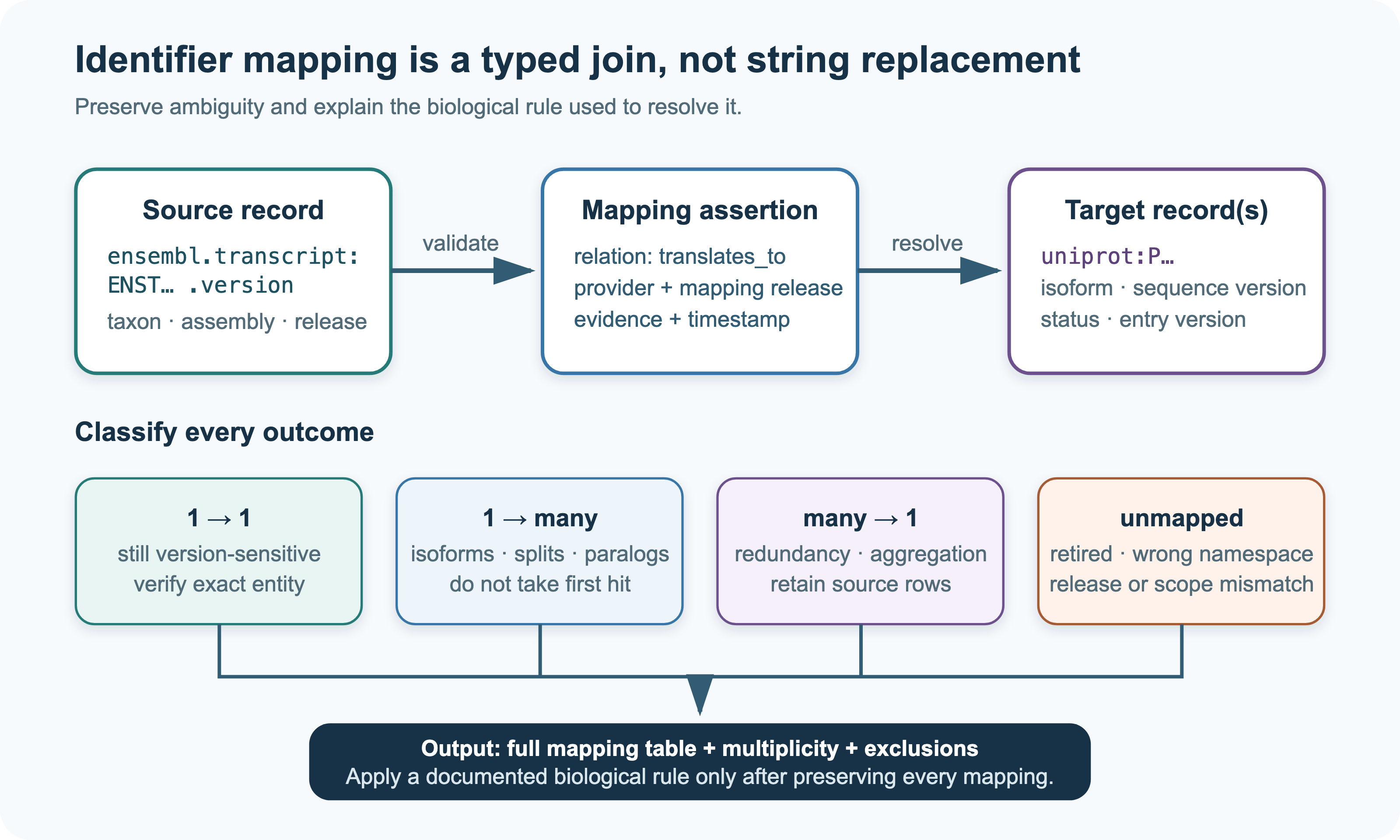
It helps to think of identifier mapping as a join between two tables rather than as replacing one string with another (Figure 2.1). Every mapping has a direction and a type (a transcript translates to a protein, a gene has a transcript), comes from a particular mapping release, and falls into one of four classes: one-to-one (still dependent on versions), one-to-many (isoforms, paralogues, split records), many-to-one (redundant records, aggregation), or unmapped (retired identifiers, the wrong namespace, a release mismatch). The rule used to resolve ambiguous cases should depend on the question: summing transcripts to genes may be right for gene-level expression, but it destroys the object of study in an analysis of isoform-specific function. Taking the first hit is never a rule.

Figure 2.1: Identifier mapping as a typed join. A source record (here an Ensembl transcript with its version) is mapped through an explicit relation, with its provider and release, to one or more target records (here UniProt entries). Every outcome is classified, and the full mapping table, including multiple mappings and failures, is kept. Figure: Matteo Tadiello, Modern Bioinformatics: From Foundations to Frontiers (CC BY 4.0).

Three further pitfalls are common:

  • An accession only means something within its namespace: P04637 is a UniProt accession, GO:0006915 a GO term. Compact identifiers of the form prefix:accession (for example uniprot:P04637) make the namespace explicit and can be resolved by services such as Identifiers.org (Wimalaratne et al. 2018).
  • A genomic coordinate is not an identifier. chr7:117,559,590 is ambiguous without the assembly (GRCh37 or GRCh38), the contig accession, whether positions are counted from 0 or 1, and how the alleles are written (Section 2.4). Converting coordinates between assemblies is a transformation that can fail, not a lookup.
  • Spreadsheets corrupt identifiers. Opened in a spreadsheet program, gene symbols such as SEPT2 or MARCH1 were silently converted into dates, and long numeric identifiers into floating-point numbers. A survey found such errors in about a fifth of the papers whose supplementary spreadsheets contained gene lists (Ziemann et al. 2016); HGNC has since renamed the affected genes (to SEPTIN2 and MARCHF1). Identifiers should be kept as text, and ideally not handled in spreadsheets at all.

2.2.5 Retrieval: Entrez, EBI Search and APIs

The large data centres provide integrated search systems over all their databases.

  • Entrez is NCBI’s search system. It links some 40 databases (nucleotide, protein, gene, genome, structure, taxonomy, PubMed and others) so that one can move from a paper to the sequences it describes, and from a gene to its protein, variants and structures (Sayers et al. 2024).
  • EBI Search plays the same role for the resources at EMBL-EBI (ENA, UniProt, InterPro, PDBe, Ensembl, Expression Atlas and many others).
  • Almost every major database also has a programmatic interface (API), usually a REST service that returns data in JSON or a standard file format. Examples are NCBI’s E-utilities, the UniProt and Ensembl REST APIs, and the RCSB PDB search and data APIs. Programmatic access is how large analyses are done, and it makes them easier to reproduce, because the exact query and database release can be recorded (Programming and reproducible research).

Many resources can also be downloaded in full. For large analyses this is often the best option, since it fixes the database version used.

A programmatic query should be treated like any other method. Record the literal query, the filters and the date; check that the number of records retrieved matches the number the server reports (results usually come in pages, and an interrupted download is easy to miss); keep the raw responses; and respect the service’s usage rules. NCBI’s E-utilities, for example, allow three requests per second without an API key and ten with one. Documented APIs and bulk downloads are preferable to extracting data from web pages, whose layout can change at any time.

2.2.6 Releases, versions and reproducibility

Databases are not fixed objects. UniProt, Pfam, Ensembl, GENCODE and most other resources appear in numbered or dated releases, and between releases entries are added, corrected, merged and deleted. The same query can therefore give different answers a year apart. A BLAST E-value depends on the size of the database searched (Section 1.2), a GO enrichment depends on the annotations in that release, and the 2025 reduction of UniProtKB (Section 2.3) changed the content of every search against it. The database release, or the download date for resources without releases, is therefore part of every computational result, in the same way as the software version and the parameters. Record it in the methods, and keep or deposit the exact files used when the analysis must be reproducible (Programming and reproducible research).

2.2.7 Licences, FAIR data and access

Most core resources are free to use, but their licences differ. INSDC data carry no restrictions on use, PDB data are released under CC0, and UniProt under CC BY 4.0, which requires attribution. Some resources, such as KEGG (Section 2.6), OMIM and COSMIC (Section 2.9), are free to browse but require a licence for bulk download or commercial use. The licence matters when data are redistributed, for example as part of a derived database or a training set for a machine-learning model.

The FAIR principles state that data should be findable, accessible, interoperable and reusable (Wilkinson et al. 2016). In practice this means persistent identifiers, rich metadata, standard formats and vocabularies (such as the ontologies in Section 2.6) and a clear licence. FAIR does not mean open: data can be FAIR and still be under controlled access. Human genetic and health data are the main example. They are deposited in controlled-access archives such as dbGaP and EGA, where use is limited by the consent of the participants (Section 2.9).

2.2.8 The literature: PubMed, PMC and preprints

The scientific literature is itself a database. PubMed, run by NCBI, indexes the biomedical literature from MEDLINE and other sources: about 41 million records in October 2026. Records are indexed with Medical Subject Headings (MeSH), and searches can be combined with Boolean operators (AND, OR, NOT) and exact phrases in quotation marks. PubMed Central (PMC) is the free full-text archive, with about 12.7 million articles, roughly a third of PubMed. Preprint servers, above all bioRxiv for biology, make papers available before peer review. Preprints are now a normal part of the literature in bioinformatics, but they have not been reviewed and should be read with that in mind.

Every January, Nucleic Acids Research publishes a database issue with papers on new and updated databases (182 papers in 2026), and maintains a collection of more than 2,000 molecular biology databases (Rigden and Fernández 2025). It is the best place to find the current description of nearly every resource in this chapter.

2.2.9 Choosing a resource for a question

The rest of this chapter goes through the resources by data type. In practice the choice starts from the question, and each question has its own pitfalls:

Question Where to start What to check
What sequence was submitted? INSDC: GenBank, ENA, DDBJ (Section 2.3) Accession and version, sample metadata, contamination
What is the reference transcript or protein? RefSeq, Ensembl (Section 2.4) Assembly and annotation release, transcript version, MANE status
What is known about a protein? UniProtKB Reviewed or not, which isoform, evidence for each statement
Which domains or families does it contain? InterPro and its member databases Which method, match coordinates and thresholds, architecture
Is there an experimental structure? PDB (Section 2.5) Method, resolution and validation, construct, biological assembly
Is there a predicted structure? AlphaFold DB and other model archives That it is a prediction; model version; pLDDT and PAE
What does it do, in which pathway? GO, Reactome, KEGG (Section 2.6) Evidence codes, ontology release, whether pathway membership was transferred from another species
What does it interact with? IntAct, BioGRID, STRING (Section 2.7) Physical interaction or functional association; evidence type
Where and when is it expressed? GEO, Expression Atlas, GTEx (Section 2.8) Study design, sample metadata, raw versus processed data
Is a variant common, and has it been interpreted? gnomAD, ClinVar (Section 2.9) Ancestry and coverage; review status, condition and conflicts

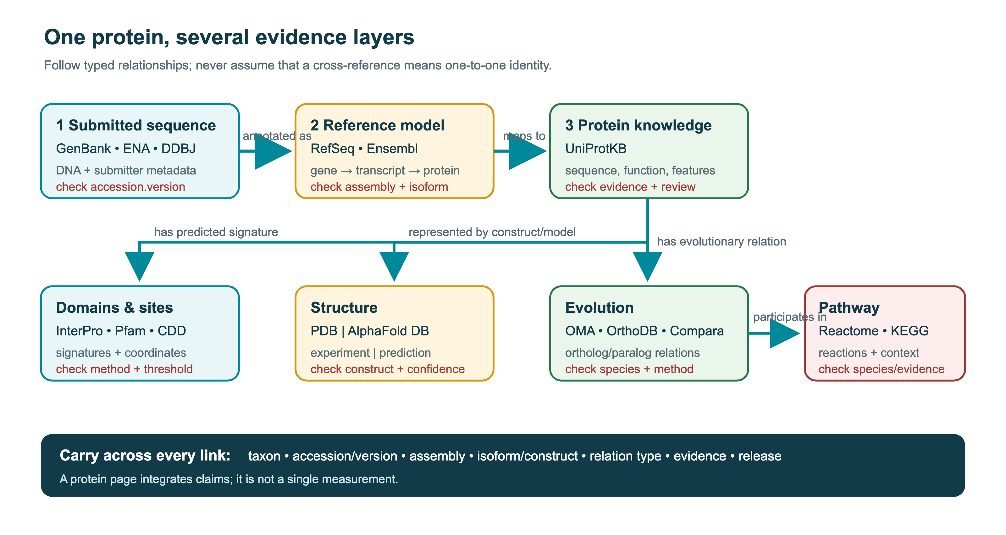
The same molecule is represented differently in each of these resources (Figure 2.2). A submitted genomic sequence can give several transcripts; the canonical UniProt sequence need not be the construct that was crystallised; a pathway assignment may have been inferred from another species. The organism, accession and version, assembly, isoform or construct, the type of each link and the release must therefore be carried along at every step. The question is not just “where is this protein?” but “which representation of this protein supports which claim?”

Figure 2.2: One protein seen through several evidence layers: the submitted sequence, the reference gene, transcript and protein models, the UniProtKB entry, and from there domains and sites, experimental or predicted structures, orthologues and pathways. The arrows are typed relationships, not statements that the records are identical. Figure: Matteo Tadiello, Modern Bioinformatics: From Foundations to Frontiers (CC BY 4.0).

See also: further explanation in Section D.2.1; related Wikipedia articles in Section E.2.1.

NoteSources

Parts of this section are adapted from the Wikipedia articles Biological database, Accession number (bioinformatics), Entrez and PubMed (CC BY-SA 4.0, retrieved 2 October 2026). The structure and the β-globin example follow the database session of the KB8029 course book. Counts were retrieved from the NCBI E-utilities on 2 October 2026. Parts of this section are adapted from Matteo Tadiello, Modern Bioinformatics: From Foundations to Frontiers, chapter “Biological Data, Databases, and Provenance” (CC BY 4.0), used with permission.

2.3 Sequence databases

2.3.1 The nucleotide archives: INSDC

All published nucleotide sequences are archived by the International Nucleotide Sequence Database Collaboration (INSDC) (Arita et al. 2020). It has three partners, which exchange their data every day so that the same records are available from all three:

  • GenBank at NCBI in the USA, founded in 1982 at Los Alamos;
  • the European Nucleotide Archive (ENA) at EMBL-EBI in the UK, whose predecessor, the EMBL Data Library, started in 1980;
  • the DNA Data Bank of Japan (DDBJ), founded in 1986.

INSDC is therefore one shared collection with three access points, not three independent databases: searching or counting all three gives the same records, not three times as many. Researchers submit to any of the three, and the record receives an accession number that is valid in all. The archives are not curated in the sense of being corrected by the database. An INSDC record is the submitter’s sequence and annotation, and stays that way unless the submitter updates it. Data are free to use without restriction. The archives have grown with sequencing technology: GenBank release 271 (April 2026) contained more than 50 trillion bases in over six billion records, most of them from whole-genome shotgun and other bulk projects.

Raw sequencing data are kept separately, in the Sequence Read Archive (SRA) at NCBI and in ENA, which also mirror each other. A sequencing study is organised in a hierarchy of study, sample, experiment and run records, so that reads can be traced back to the biological samples they came from. Assembled genomes, transcriptome assemblies, and metadata about samples (BioSample) and projects (BioProject) are linked to the reads. Raw data are essential for reanalysis, but they are now so large that the archives store some of them in compressed or reduced forms.

2.3.2 Curated nucleotide and gene resources

Because the archives contain many redundant, partial and differently annotated records, curated resources have been built on top of them. RefSeq at NCBI, started in 2000, is such a secondary resource, not part of the INSDC archive. It provides a single, non-redundant, annotated record for each genomic sequence, transcript and protein of a selected organism (O’Leary et al. 2015). The accession prefix shows the type of molecule: NC_ (complete chromosome), NM_ (mRNA), NR_ (non-coding RNA), NP_ (protein), and XM_/XP_ for transcripts and proteins predicted by the annotation pipeline but not yet supported by curated evidence. NCBI Gene collects information about each gene, and Ensembl provides the European counterpart for genomes and their annotation (Section 2.4).

2.3.3 Protein sequences: UniProt

Almost no protein sequences are determined directly any more. They are translated from genes predicted in sequenced genomes. UniProt, the Universal Protein Resource, is the central database for protein sequences and their functions (Bateman et al. 2024). It was formed in 2002 by combining three older resources: Swiss-Prot, started by Amos Bairoch in 1986 in Geneva; its automatically annotated supplement TrEMBL (1996); and the Protein Information Resource (PIR), the descendant of Margaret Dayhoff’s Atlas of Protein Sequence and Structure. It is run by EMBL-EBI, the Swiss Institute of Bioinformatics and PIR. Its main parts are:

  • UniProtKB/Swiss-Prot: manually reviewed entries. Curators read the literature, record function, catalytic activity, subcellular location, domains, post-translational modifications, variants and disease associations, and merge all sequences of the same protein from one species into one entry. About 576,000 entries (release 2026_03).
  • UniProtKB/TrEMBL: unreviewed entries, annotated automatically by rule-based systems (UniRule, ARBA) that transfer annotation from reviewed entries to proteins of the same family. About 149 million entries (release 2026_03).
  • UniParc: an archive in which every unique protein sequence from any source appears exactly once, under a stable identifier. It contains more than a billion sequences (2026).
  • UniRef: clusters of UniProt and selected UniParc sequences at 100%, 90% and 50% identity (UniRef100, UniRef90, UniRef50) (Suzek et al. 2014). Searching UniRef instead of the full database removes most redundancy and is much faster. UniRef50 was, for example, used to train protein language models (Section 1.10).
  • Proteomes: the set of proteins of each sequenced organism, with a selected reference proteome for each species or strain.

The difference in quality between the two sections of UniProtKB is large. A Swiss-Prot entry is a short review of what is experimentally known about a protein. A TrEMBL entry is a prediction: its sequence depends on an automatic gene model, and its annotation is inferred from homologues. The size of UniProtKB also depends on policy. To limit redundancy, UniProt decided in 2025 to keep only proteins from reference proteomes in UniProtKB, unless there is a specific reason to keep an entry, for example an experimental structure. This reduced UniProtKB from about 250 million to about 150 million entries during 2025–2026. The removed sequences remain available in UniParc.

2.3.4 Metagenomic sequences

A growing share of all known protein sequences comes not from cultured organisms but from metagenomes: DNA sequenced directly from environmental or host-associated samples. Most of these sequences are not in UniProtKB. MGnify at EMBL-EBI assembles and annotates metagenomic data and provides a protein database with billions of sequences (Richardson et al. 2022). Clustered collections of metagenomic and genomic proteins, such as the Big Fantastic Database (BFD) and the databases built with Linclust (Section 1.4), are used to build the deep multiple alignments needed for structure prediction (Chapter 9). Metagenomic proteins have also been predicted structurally on a massive scale (Section 2.5).

2.3.5 Protein families and domains

Family and domain databases classify sequences by homology. They are described in detail in Section 1.9 and are listed here only for completeness:

  • Pfam: families and domains defined by curated seed alignments and profile HMMs, now including deep-learning annotations (Pfam-N) (Mistry et al. 2020; Paysan-Lafosse et al. 2024).
  • InterPro: integrates Pfam and about a dozen other signature databases (PROSITE, SMART, PANTHER, CDD, NCBIfam, CATH-Gene3D, SUPERFAMILY and others) into a single classification. Its matches are precomputed for all of UniProtKB (Blum et al. 2024).
  • SCOP, CATH, ECOD and TED: classifications of domains of known or predicted three-dimensional structure (Section 2.5).
  • Rfam: the corresponding database for families of non-coding RNAs (Section 1.7).

See also: further explanation in Section D.2.2; related Wikipedia articles in Section E.2.2.

NoteSources

Parts of this section are adapted from the Wikipedia articles International Nucleotide Sequence Database Collaboration, GenBank, European Nucleotide Archive, Sequence Read Archive, RefSeq and UniProt (CC BY-SA 4.0, retrieved 2 October 2026). UniProt counts were retrieved from the UniProt REST API (release 2026_03) on 2 October 2026.

2.4 Genome databases and browsers

A genome sequence becomes useful when it is annotated: genes, transcripts, regulatory elements, variants and comparisons with other species have to be placed on the sequence and kept up to date as assemblies improve. Genome browsers present this information graphically, as tracks along a chromosome, and are among the most used tools in biology.

  • Ensembl was started in 1999 by EMBL-EBI and the Sanger Institute to annotate the human genome automatically as it was being sequenced (Dyer et al. 2024). It now covers hundreds of vertebrate genomes, with gene models built by an automatic pipeline from aligned transcripts and proteins, combined with manual annotation (GENCODE) for human and mouse. It also provides comparative genomics (orthologues, paralogues and whole-genome alignments), variation data and the Variant Effect Predictor. Ensembl Genomes extends the system to bacteria, fungi, plants, protists and invertebrates. Ensembl is moving to a new browser and data model designed for many more genomes.
  • The UCSC Genome Browser, from the University of California, Santa Cruz, displayed the first working draft of the human genome in 2000 (Perez et al. 2024). It is known for its large collection of annotation tracks contributed by many projects (conservation, regulatory elements, expression, variation, repeats), its fast display, and tools such as BLAT (Section 1.4) and the Table Browser. Users can upload their own data as custom tracks.
  • NCBI provides the Genome, Gene and RefSeq resources and its own Genome Data Viewer, together with the annotation pipelines that produce the RefSeq gene models for eukaryotes and prokaryotes (Sayers et al. 2024).

Ensembl, UCSC and NCBI annotate the human genome independently. Their gene sets largely agree, and the MANE project (Matched Annotation from NCBI and EMBL-EBI) now defines one agreed reference transcript per human protein-coding gene, which is important for reporting clinical variants consistently. The coordinates of features depend on the genome assembly (for example GRCh37/hg19 or GRCh38/hg38 for human), so the assembly version must always be stated. Converting coordinates between assemblies (“liftover”) is a common source of errors. The first complete telomere-to-telomere human genome (T2T-CHM13) and the human pangenome reference are gradually being added to these resources (Chapter 5).

2.4.1 Annotation formats and coordinates

Features on a genome, such as genes, exons, peaks or variants, are exchanged as tables of coordinates. Two families of formats dominate, and they count positions differently.

  • BED (Browser Extensible Data), from UCSC, has three required columns (chromosome, start, end) and up to nine optional ones (name, score, strand, the coding region, colour, and the sizes and starts of blocks such as exons). It is compact and is the input of tools such as BEDTools (Quinlan and Hall 2010), which intersect, merge and compare sets of intervals.
  • GFF3 (General Feature Format) has nine columns: sequence, source, feature type, start, end, score, strand, phase (the reading frame of a CDS) and free-form attributes. Feature types are terms from the Sequence Ontology, and the ID and Parent attributes link exons and CDSs to transcripts and transcripts to genes, so that a whole gene model can be described. GTF is an older dialect (GFF version 2) with mandatory gene_id and transcript_id attributes, still used by Ensembl and GENCODE and by most RNA-seq quantification tools (Chapter 7).

The two families also use different coordinate conventions. BED is 0-based, half-open: the first base of a chromosome is position 0, and the interval \([s, e)\) includes the start but not the end, so its length is \(e - s\). GFF3, GTF, VCF and SAM are 1-based, closed: the first base is 1, and \([s, e]\) includes both ends, so the length is \(e - s + 1\). The same single base, the 100th of chromosome 1, is therefore written chr1 99 100 in BED and as start = end = 100 in GFF. Converting between the two means subtracting 1 from the start and leaving the end unchanged. The UCSC browser displays 1-based coordinates but stores 0-based ones, and BAM files store 0-based positions that are displayed as 1-based SAM. Forgetting a conversion gives off-by-one errors: features shifted by one base, zero-length or one-base-too-long intervals, and variants assigned to the wrong base or the wrong codon. Such errors are silent: the files still parse, and the results are almost right. A related source of silent failure is chromosome naming (chr1 at UCSC, 1 at Ensembl), which can make two files that describe the same genome share no features at all.

Coordinates also only mean something together with the genome build, the assembly version they refer to (Section 2.2). Human GRCh37 is the same assembly as UCSC’s hg19, and GRCh38 the same as hg38; the positions of most features differ between them, sometimes by megabases. Liftover converts coordinates from one build to another using a whole-genome alignment of the two assemblies, stored as chain files (Section 1.8), with UCSC liftOver or CrossMap (Zhao et al. 2013). Liftover is a transformation, not an identity: some regions cannot be converted because they were changed, added or removed in the new assembly, others are split or map to several places, and alleles may differ when the reference base has changed. For important analyses it is better to map the original reads to the new assembly than to lift over the results.

2.4.2 Organism-specific databases

For each major model organism there is a dedicated model organism database, curated by experts who follow the literature on that organism. Examples are SGD (budding yeast), PomBase (fission yeast), FlyBase (Drosophila), WormBase (C. elegans), ZFIN (zebrafish), MGI (mouse), RGD (rat), TAIR (Arabidopsis) and EcoCyc (E. coli). They hold gene nomenclature, mutant phenotypes, genetic and physical interactions, and detailed functional annotation that the general databases often import. Several of them are federated in the Alliance of Genome Resources. For prokaryotes, collections of genomes and taxonomies such as NCBI’s prokaryotic RefSeq and the Genome Taxonomy Database (GTDB), which classifies bacteria and archaea by genome phylogeny, are the most important resources (Chapter 6).

2.4.3 Taxonomy databases

Almost every database record carries the organism it came from, and the taxonomy is the key that links them. NCBI Taxonomy (Schoch et al. 2020) holds the names and classification of all organisms with sequences in INSDC (Section 2.3), each identified by a numerical taxid (9606 for Homo sapiens, 562 for Escherichia coli). The taxid, not the name, is what UniProt, RefSeq, Ensembl, the PDB and many other resources use to say which organism an entry belongs to, and it is how searches can be restricted to a clade (for example, BLAST against Metazoa only). Names change and can be ambiguous; taxids are stable, although they can be merged or deleted when the classification is revised. The NCBI database explicitly states that it is not an authoritative source for nomenclature or classification: it is a curated working classification that follows the literature and taxonomic experts, and it contains many provisional names for unclassified and environmental organisms.

For bacteria and archaea, the Genome Taxonomy Database (GTDB) (Parks et al. 2018, 2021) offers an alternative: a classification derived entirely from a phylogeny of conserved single-copy proteins of genomes, including metagenome-assembled genomes, with ranks normalised by evolutionary divergence. It reclassified many groups and renamed many taxa, so the same genome can have different names in NCBI and GTDB. The principles behind the two approaches are discussed in Section 4.5.

See also: further explanation in Section D.2.3; related Wikipedia articles in Section E.2.3.

NoteSources

Parts of this section are adapted from the Wikipedia articles Ensembl genome database project, UCSC Genome Browser and Model organism database (CC BY-SA 4.0, retrieved 2 October 2026). The subsections on annotation formats and taxonomy databases were written for this book from the primary literature cited in the text.

2.5 Structure databases

Structure resources fall into two groups that should not be confused: the PDB, an archive of structures determined by experiment, and collections of computationally predicted models, such as the AlphaFold database.

2.5.1 The Protein Data Bank: experimental structures

The Protein Data Bank (PDB), founded in 1971 at Brookhaven National Laboratory with seven structures, is the single global archive of experimentally determined structures of proteins, nucleic acids and their complexes (Berman et al. 2000; Burley et al. 2018). Since 2003 it has been managed by the worldwide PDB (wwPDB): RCSB PDB in the USA, PDBe in Europe, PDBj in Japan, the Biological Magnetic Resonance Data Bank (BMRB) and, since 2021, the Electron Microscopy Data Bank (EMDB). Depositions are processed and validated by curators, and the data are freely available under a CC0 licence. In October 2026 the PDB contained about 260,000 experimental structures.

Each entry contains the atomic coordinates, the experimental data (such as structure factors for X-ray crystallography or restraints for NMR), information about the sample and the method, and a validation report that compares the model with the data and with expected geometry. Quality varies a lot between entries. For crystal structures, the resolution and the R and R-free values are the first things to check (Brünger 1992). Note also that the deposited asymmetric unit is not necessarily the biologically relevant assembly, which is given separately. The standard file format is now PDBx/mmCIF, which has replaced the old fixed-column PDB format because that format cannot represent very large structures. Integrative (or hybrid) structures, which combine data from several experimental methods with computational modelling, use an extension of PDBx/mmCIF and are archived through PDB-IHM (formerly PDB-Dev), now part of the wwPDB. They are experimentally based, but their precision is often lower than that of a crystal or cryo-EM structure.

EMDB archives the three-dimensional density maps from cryo-electron microscopy and tomography (Turner et al. 2023). The atomic models built into the maps are deposited in the PDB. With the rapid growth of cryo-EM, an increasing share of new structures, especially of large complexes and membrane proteins, comes from EMDB/PDB pairs.

Structures are classified into domains, folds and superfamilies by SCOP, CATH and ECOD, and the domains of predicted structures by TED (Section 1.9).

2.5.2 Predicted structures: model databases

Since 2021, predicted structures have become a resource in their own right, much larger than the PDB. These are prediction resources, not archives of experimental data, and purely computational models are not accepted in the PDB. They are models, not measurements, and must always be used together with their confidence estimates (pLDDT and predicted aligned error, PAE; Chapter 9).

  • The AlphaFold Protein Structure Database (AFDB), built by DeepMind and EMBL-EBI, was released in July 2021 with the proteomes of humans and 20 model organisms, and expanded in 2022 to more than 200 million proteins, almost all of UniProt (Varadi et al. 2021, 2023). In 2025 it was updated to a recent UniProt release, with a redesigned interface, isoforms and domain annotations (Bertoni et al. 2025). In 2026 it started to include predicted complexes: about 80,000 high-confidence heterodimers and 1.7 million homodimers, mainly from about 20 well-studied species and priority pathogens, with millions of lower-confidence predictions available for download.
  • The ESM Metagenomic Atlas contains more than 600 million structures of metagenomic proteins, predicted with ESMFold (Lin et al. 2023). Most of these proteins are from organisms that have never been cultured.
  • AFDB does not cover viral proteins. The Big Fantastic Virus Database (BFVD), from Martin Steinegger’s group, fills this gap with structures of viral proteins predicted with ColabFold (Kim et al. 2024). Its first version contained about 350,000 structures of representative sequences. Many of them have no structural similarity to anything in the PDB or AFDB, and later versions cover almost all viral proteins in UniProt.
  • Other collections of models (ModelArchive, SWISS-MODEL Repository) are linked to the PDB and AFDB through the 3D-Beacons network, so that experimental and predicted models of a protein can be found in one place.

These collections are only searchable at this scale because of fast structure-search tools such as Foldseek, which also made it possible to cluster the whole AFDB and discover new folds (van Kempen et al. 2023; Barrio-Hernandez et al. 2023) (Section 1.4).

See also: further explanation in Section D.2.4; related Wikipedia articles in Section E.2.4.

NoteSources

Parts of this section are adapted from the Wikipedia articles Protein Data Bank, EM Data Bank and AlphaFold (CC BY-SA 4.0, retrieved 2 October 2026). The PDB count was retrieved from the RCSB Search API on 2 October 2026; the 2026 AFDB complexes are described in an EMBL announcement.

2.6 Function and pathways

2.6.1 The Gene Ontology

The Gene Ontology (GO), started in 1998 by the model organism databases for fly, yeast and mouse, provides a shared, controlled vocabulary for describing what genes and proteins do in any organism (Ashburner et al. 2000; The Gene Ontology Consortium et al. 2023). It has three independent parts:

  • Molecular function: the activity of the gene product at the molecular level, such as “protein kinase activity” or “ATP binding”;
  • Biological process: the larger biological programme that the activity contributes to, such as “DNA repair” or “cell division”;
  • Cellular component: where the gene product is located or acts, such as “mitochondrial inner membrane” or “ribosome”.

Terms are organised as a directed acyclic graph rather than a strict tree: a term can have several parents, linked by relations such as is_a and part_of. An annotation to a specific term implies all of its ancestors (the “true path rule”). This structure is what makes GO useful for computation, for example for enrichment analysis, where one asks whether a list of genes is annotated to some term more often than expected by chance (Section 7.4.1, Chapter 7).

Every annotation of a gene to a GO term carries an evidence code. Annotations based on experiments (for example IDA, inferred from direct assay) are distinguished from those inferred from phylogeny or sequence similarity (IBA, ISS) and from fully automatic electronic annotations (IEA), which are the large majority. As discussed in Section 2.2, the evidence code tells you how much to trust an annotation, and whether it is independent evidence or a copy of another annotation. Other classification systems used alongside GO are the Enzyme Commission (EC) numbers for enzymatic reactions and the reaction database Rhea.

2.6.2 Pathway databases

  • KEGG (Kyoto Encyclopedia of Genes and Genomes) was started in 1995 by Minoru Kanehisa at Kyoto University (Kanehisa et al. 2024). Its best-known part is a set of manually drawn pathway maps for metabolism, signalling, cellular processes and diseases. Genes are linked to the maps through KEGG Orthology (KO) groups, so that the pathways can be reconstructed automatically for any sequenced genome. KEGG also contains modules, compounds, reactions, drugs and diseases. The website is free for academic use, but bulk downloads require a licence, which is why some open tools use other resources.
  • Reactome is an open, expert-curated database of human pathways and reactions, developed by OICR, EMBL-EBI, NYU and OHSU (Milacic et al. 2023). Pathways are built from individual reactions with defined inputs, outputs, catalysts and regulators, each supported by literature references. Pathways for other species are inferred by orthology. Reactome is widely used for pathway enrichment analysis.
  • Other important resources are MetaCyc and BioCyc for metabolic pathways across organisms, WikiPathways for community-curated pathways, and BioModels for quantitative, computational models of pathways.

2.6.3 Ontologies and knowledge graphs

GO is one of many biomedical ontologies, controlled vocabularies whose terms are linked by defined relations. Others describe chemical entities (ChEBI), sequence features (Sequence Ontology), anatomy (Uberon), cell types (Cell Ontology), human phenotypes (Human Phenotype Ontology) and diseases (Mondo). Many are developed together in the OBO Foundry, so that they use compatible identifiers and relations. When databases annotate their records with the same ontology terms, the records can be combined across resources.

A knowledge graph takes this integration further. Genes, proteins, GO terms, pathways, compounds, diseases and phenotypes become nodes, and relations from many databases (a protein participates in a Reactome reaction, a gene is associated with a disease, a drug targets a protein) become typed edges. Several resources, UniProt among them, also distribute their data in this form (as RDF, queried with SPARQL). Knowledge graphs are used for queries across databases, for prioritising disease genes and for drug repurposing (Himmelstein et al. 2017), often with graph machine-learning methods (Chapter 12). They inherit the biases of their sources: well-studied genes have many more edges, and a missing edge usually means “not studied” rather than “no relation”.

2.6.4 Evaluating function prediction: CAFA

Because most annotations are predictions, it matters how good the prediction methods are. The Critical Assessment of Functional Annotation (CAFA) evaluates them prospectively. Participants predict GO terms for thousands of proteins without experimental annotation, and the predictions are scored against the experimental annotations that accumulate in the following months (Radivojac et al. 2013; Zhou et al. 2019). The fifth round (CAFA5) was run as a Kaggle competition with a much larger number of participants. It showed clear improvements, attributed to protein language models, predicted structures and the growth of experimental annotations (De Paolis Kaluza et al. 2026). CAFA also highlights a general problem of the field: annotations are incomplete, so a “false” prediction may simply be one that has not yet been tested (Chapter 10).

See also: further explanation in Section D.2.5; related Wikipedia articles in Section E.2.5.

NoteSources

Parts of this section are adapted from the Wikipedia articles Gene Ontology, KEGG and Reactome (CC BY-SA 4.0, retrieved 2 October 2026).

2.7 Interaction databases

Interaction databases differ in what kind of relationship they record, and this matters for how they can be used (Chapter 11).

  • Curated physical interactions. IntAct at EMBL-EBI curates molecular interactions from the literature in fine detail: the experimental method, the participants, their roles and any binding regions (Toro et al. 2021). It is the main member of the IMEx consortium, which shares a common curation standard. BioGRID, started in 2003, curates protein–protein and genetic interactions, chemical interactions and post-translational modifications for the major model organisms and human, and includes many large screens (Oughtred et al. 2020). The Complex Portal describes curated stable complexes with their composition and stoichiometry, for example the haemoglobin tetramer of two α and two β chains (Meldal et al. 2021).
  • Functional association networks. STRING combines experimental interactions with evidence from genomic context (gene neighbourhood, fusion, co-occurrence), co-expression, curated pathways and text mining, and transfers associations between organisms by orthology. Each link has a confidence score, and the network covers thousands of organisms (Szklarczyk et al. 2022, 2024). The 2025 version also distinguishes directed, regulatory links. FunCoup, developed by Erik Sonnhammer’s group in Stockholm, builds networks with a naive Bayesian framework that integrates many types of evidence, and recent versions include directed gene-regulatory links for human and many other species (Buzzao et al. 2024; Guala et al. 2019). A link in these networks means that two proteins probably work together. It does not necessarily mean that they bind each other.
  • Maps of complexes from proteomics. hu.MAP integrates thousands of affinity-purification and co-fractionation mass-spectrometry experiments with machine learning to predict human protein complexes. Version 3.0 combined more than 25,000 experiments and identified more than 15,000 complexes covering about 70% of the human proteome (Fischer et al. 2025). The complexes are also imported into the Complex Portal.
  • Predicted structures of complexes. Large sets of AlphaFold-predicted complexes are now available, including in the AlphaFold database (Section 2.5). They add a structural model and a confidence to a predicted interaction.

When using interaction data, ask what type of evidence a link is based on. High-throughput screens and text mining have different error rates, and interactions between very well-studied proteins are over-represented simply because more experiments have been done on them.

See also: further explanation in Section D.2.6; related Wikipedia articles in Section E.2.6.

NoteSources

Parts of this section are adapted from the Wikipedia articles STRING and BioGRID (CC BY-SA 4.0, retrieved 2 October 2026).

2.8 Expression and proteomics repositories

Functional genomics experiments are archived in their own primary repositories, again usually as a condition of publication.

  • GEO (Gene Expression Omnibus), at NCBI since 2000, archives microarray, RNA-seq, single-cell and epigenomics data sets, with processed data and descriptions of the samples, while the raw reads are stored in the SRA (Clough et al. 2023).
  • ArrayExpress, at EMBL-EBI since 2002, is the European counterpart. It is now part of BioStudies, a general archive for data that belong to one study, with the raw reads in ENA.
  • Curated, reanalysed views of these data are provided by, for example, the Expression Atlas and Single Cell Expression Atlas at EMBL-EBI, GTEx (gene expression across about 50 human tissues from around a thousand donors), and the Human Protein Atlas, a Swedish project started in 2003 that maps human proteins in tissues, cells and organs with antibodies, transcriptomics and other methods (Uhlén et al. 2015).
  • PRIDE at EMBL-EBI is the largest repository of mass-spectrometry proteomics data (Perez-Riverol et al. 2024). It is part of the ProteomeXchange consortium, which coordinates submission and data sharing between proteomics repositories (Chapter 8).

The value of these archives depends heavily on the metadata: which samples were compared, how they were treated and how the data were processed. Reanalysing public data is a powerful approach, but incomplete or inconsistent sample descriptions are a common obstacle. Standards such as MIAME (for microarrays) and MINSEQE (for sequencing) define the minimum information that should be provided.

See also: further explanation in Section D.2.7; related Wikipedia articles in Section E.2.7.

NoteSources

Parts of this section are adapted from the Wikipedia articles Gene Expression Omnibus and Human Protein Atlas (CC BY-SA 4.0, retrieved 2 October 2026).

2.9 Medical and variant data

Human genetic and clinical data raise two issues that the databases above do not have: the interpretation of variants for health, and the protection of personal data. The resources therefore fall into two groups: open databases of variants and their interpretation, and controlled-access archives of individual-level data.

2.9.1 Variants and their interpretation

  • dbSNP at NCBI, started in 1998, catalogues short genetic variants (single-nucleotide variants, small insertions and deletions) and gives each a stable identifier, the rs number. The European Variation Archive (EVA) plays a similar role at EMBL-EBI for variants from all species.
  • gnomAD (Genome Aggregation Database) aggregates exome and genome sequences from large studies to provide allele frequencies in different populations. Version 4 contains data from more than 800,000 individuals (Chen et al. 2023). Its main use is to tell whether a variant is rare or common, and which genes tolerate loss-of-function variants (constraint), which is essential when judging whether a variant could cause a rare disease. The 1000 Genomes Project produced an earlier, openly accessible reference of human genetic variation.
  • ClinVar at NCBI collects interpretations of variants submitted by clinical laboratories and researchers, classified on a scale from benign to pathogenic, together with the supporting evidence (Landrum et al. 2017). Most clinical laboratories classify variants with the ACMG/AMP guidelines, which combine population frequency, segregation, functional data and computational predictions (Richards et al. 2015). A ClinVar classification is therefore a submitter’s interpretation, not an experimentally established fact. Conflicting interpretations between submitters are common and are shown explicitly, and each record has a review status (zero to four stars), from a single submitter without stated criteria to an expert panel or practice guideline. Classifications also change over time, often from uncertain significance to benign or pathogenic. When ClinVar is used as a ground truth, for example to train or evaluate variant effect predictors, the review status should be filtered, the release recorded, and circularity with computational evidence kept in mind (Section 10.6, Section 12.2).
  • OMIM (Online Mendelian Inheritance in Man) is the classic curated catalogue of human genes and genetic disorders, going back to Victor McKusick’s Mendelian Inheritance in Man from the 1960s (Amberger et al. 2018).
  • The GWAS Catalog (NHGRI and EMBL-EBI) collects the associations between variants and traits reported in genome-wide association studies (Sollis et al. 2022).
  • Computational predictions of variant effects, for example AlphaMissense predictions for all possible human missense variants (Cheng et al. 2023), are integrated into several of these resources (Chapter 10).

These resources answer different questions, and mixing them up is a common error. An rs number in dbSNP shows that a variant has been observed before, not that it is benign. gnomAD gives its frequency in the sampled populations; it is not a collection of healthy controls (its cohorts include people with common diseases), and a variant’s absence from gnomAD is weak evidence if coverage at that position is poor or the relevant ancestry is under-represented. ClinVar records interpretations for a stated condition and mode of inheritance, which should be read together with their review status and dates rather than counted as votes. All three depend on the reference assembly and on the transcript used to describe the variant: the same genomic change can have different consequences in different transcripts, and GRCh37 and GRCh38 coordinates must never be mixed.

2.9.2 Cancer genomics

  • The Cancer Genome Atlas (TCGA), a project of the US National Cancer Institute and NHGRI from 2006, characterised more than 11,000 tumours from 33 cancer types with genome, exome, transcriptome, methylation and protein data (Weinstein et al. 2013). Its data, and those of later projects, are distributed through the NCI Genomic Data Commons (GDC). The International Cancer Genome Consortium (ICGC) coordinated similar projects worldwide.
  • COSMIC (Catalogue of Somatic Mutations in Cancer), at the Sanger Institute since 2004, is an expert-curated database of somatic mutations in cancer, including the Cancer Gene Census of genes with a documented role in cancer (Sondka et al. 2023).

2.9.3 Controlled access to personal data

Sequences and clinical data from individual people can identify them, so they are not openly published. They are deposited in controlled-access archives, such as dbGaP at NCBI and the European Genome-phenome Archive (EGA) at EMBL-EBI and CRG in Barcelona. Researchers must apply to a data access committee and agree to conditions on how the data are used and stored. The permitted uses follow from the consent the participants gave: a data set may be restricted to research on a particular disease, to non-commercial use, or to approved projects only. These restrictions travel with the data and also apply to any derived data set. In Europe, the use of such data is regulated by the General Data Protection Regulation (GDPR); in Sweden, research on personal data also requires ethical approval (Programming and reproducible research). Large biobanks, such as the UK Biobank with genetic and health data from about half a million participants, are accessed in the same way, increasingly through secure analysis environments where the data never leave the provider.

Controlled access is compatible with the FAIR principles (Section 2.2): the existence and description of a data set can be open even when the data themselves are not. The CARE principles (collective benefit, authority to control, responsibility and ethics) complement FAIR for Indigenous data governance (Carroll et al. 2020). They stress that the peoples and communities from which data come should have a say in how the data are used and should benefit from that use.

This area changes particularly quickly, and many national resources (for example for Swedish health data) are not covered here. For a current picture, start from the NAR database issue (Rigden and Fernández 2025) and the websites of the resources themselves.

See also: further explanation in Section D.2.8; related Wikipedia articles in Section E.2.8.

NoteSources

Parts of this section are adapted from the Wikipedia articles dbSNP, ClinVar, Online Mendelian Inheritance in Man, GWAS catalog, The Cancer Genome Atlas, COSMIC cancer database and European Genome-phenome Archive (CC BY-SA 4.0, retrieved 2 October 2026). Parts of this section are adapted from Matteo Tadiello, Modern Bioinformatics: From Foundations to Frontiers, chapter “Biological Data, Databases, and Provenance” (CC BY 4.0), used with permission.

2.10 Key concepts

A checklist for revision.

  • Principles: primary archives vs. curated knowledgebases vs. derived resources (GenBank vs. RefSeq, Swiss-Prot vs. TrEMBL); the DNA–RNA–protein organisation; curation vs. automatic annotation; error propagation and evidence codes; redundancy and non-redundant sets; records as versioned claims (data, metadata, knowledge assertions); why agreeing databases are not independent evidence; absence of a record is not absence; testing robustness to the evidence policy
  • Identifiers and retrieval: stable accessions vs. versioned accessions vs. names and symbols; persistent identifiers (DOI); cross-references and identifier mapping as a typed join (one-to-one, one-to-many, many-to-one, unmapped); namespaces and compact identifiers; why a genomic coordinate is not an identifier; spreadsheet corruption of gene symbols; Entrez, EBI Search and REST APIs; recording queries and checking that retrieval is complete; choosing a resource from the question; PubMed, MeSH, PMC and preprints; the NAR database issue
  • Releases and reuse: the database release as part of every result; licences (CC0, CC BY, restricted bulk download); the FAIR principles; FAIR is not the same as open
  • Sequences: INSDC (GenBank, ENA, DDBJ): one shared collection, exchanged daily; SRA and the study–sample–experiment–run hierarchy; RefSeq and its accession prefixes; UniProtKB/Swiss-Prot vs. TrEMBL, UniParc, UniRef and reference proteomes; metagenomic sequence collections (MGnify); family databases (Pfam, InterPro)
  • Genomes: Ensembl, UCSC and NCBI; gene models and MANE; BED vs. GFF3/GTF; 0-based half-open vs. 1-based closed coordinates and off-by-one errors; chromosome naming; genome builds (GRCh37/hg19, GRCh38/hg38) and liftover with chain files, and why it can fail; model organism databases
  • Taxonomy: NCBI Taxonomy and taxids as the organism key across databases (and not an authoritative nomenclature); GTDB’s genome-based, rank-normalised classification of bacteria and archaea; why the same genome can have different names
  • Structures: the PDB and wwPDB as the archive of experimental structures (integrative structures in PDB-IHM); what an entry contains, validation, resolution and R-free, asymmetric unit vs. biological assembly; mmCIF; EMDB; predicted models in AlphaFold DB (including complexes), ESM Atlas and BFVD; confidence measures of predicted models
  • Function and pathways: the three GO aspects, the GO graph and the true path rule, evidence codes; EC numbers; KEGG (pathway maps, KO) and Reactome (reactions); other ontologies (OBO Foundry) and knowledge graphs; CAFA and why function prediction is hard to evaluate
  • Interactions: curated physical interactions (IntAct/IMEx, BioGRID, Complex Portal) vs. functional association networks (STRING, FunCoup) vs. complex maps (hu.MAP); what a link means
  • Expression and proteomics: GEO, ArrayExpress/BioStudies, Expression Atlas, GTEx, Human Protein Atlas; PRIDE and ProteomeXchange; the importance of metadata
  • Medical data: dbSNP, gnomAD, ClinVar (submitted interpretations, review status, conflicts); observation vs. frequency vs. interpretation, and why gnomAD is not a set of healthy controls, OMIM, GWAS Catalog; TCGA/GDC and COSMIC; controlled access (dbGaP, EGA) and consent-based use restrictions, GDPR and ethical approval; the CARE principles

2.12 Background reading (open access)

Descriptions of Wikipedia articles are taken from the introductions of the articles (CC BY-SA 4.0).

2.13 Student recommendations

Recommended by students preparing for the exam: papers, reviews, online lectures, tutorials and short explanations. To suggest something, use the suggestion form (SU login).

No recommendations yet.

2.14 Review problems

These problems are adapted from Matteo Tadiello, Modern Bioinformatics: From Foundations to Frontiers (CC BY 4.0), used with permission. For a longer treatment of this topic, see the chapter “Biological Data, Databases, and Provenance” of that book. In the HTML version, click a box to show the extensions, solution outline and common errors.

2.14.1 Archival, derived and integrated resources

Distinguish the archival, curated, derived and integrated roles of biological databases. Explain why these roles are not a ranking of how reliable the data are.

Extensions:

  • Classify the different kinds of information in UniProtKB, RefSeq and Ensembl, rather than giving each resource a single label.
  • What happens when an integrated database copies an annotation from another integrated database?

Solution outline:

  1. Define the labels as roles: archival (primary) resources preserve submitted observations; curated and derived resources select, transform, predict or interpret them; integrated resources link many kinds of entities and evidence.
  2. One resource can play several roles. UniProtKB stores sequences translated from the nucleotide archives, computes automatic annotation (TrEMBL), curates the literature (Swiss-Prot) and integrates cross-references.
  3. Contrast submission to GenBank, ENA and DDBJ with the selection and curation of RefSeq and the computed, integrated genome annotation of Ensembl.
  4. “Primary” is not a quality label: archived data can contain submitter errors and contamination, while derived data add value but also assumptions.
  5. Trust depends on tracing the specific claim back through its evidence, transformations and versions. Copying between resources does not create independent support.

Common errors:

  • Treating “archival” as meaning “experimentally proven”.
  • Forcing every resource into one category.
  • Counting three database pages that show the same annotation as three independent observations.

Connections: Section 2.2; annotation by similarity (Section 1.4); evidence for protein function (Section 10.4).

2.14.2 Identifiers, versions and mappings

Explain why a gene symbol is not enough for reproducible bioinformatics, and describe how identity can be preserved across resources and releases.

Extensions:

  • Distinguish an accession from a versioned accession.
  • Map an Ensembl transcript to a UniProt entry while keeping one-to-many results.
  • Explain why a genomic coordinate is not a stable identifier.

Solution outline:

  1. Gene symbols are labels for people. They can be ambiguous, have aliases, be reused or change, and an identifier means something only within its namespace.
  2. A stable accession identifies a record; the version identifies one particular sequence. Record the database release and the retrieval date as well.
  3. A coordinate needs the assembly, the contig accession, the coordinate convention (0- or 1-based) and the allele representation. Liftover between assemblies is a transformation, not an identity.
  4. Treat mapping as a typed join: source accession and version, the relation, target accession and version, organism, and the source and release of the mapping.
  5. Keep one-to-many and many-to-one mappings, find out whether they reflect isoforms, paralogues, merges or splits, and choose a rule that fits the question. Never silently take the first result.
  6. Report how many identifiers mapped multiply or not at all.

Common errors:

  • Removing version suffixes without recording it.
  • Assuming that the “canonical” transcript is the dominant one in every tissue.
  • Using gene symbols as keys in spreadsheets.
  • Treating every cross-reference as an equivalence.

Connections: Section 2.2; gene models and assembly versions (Section 2.4, Section 5.6); summing transcripts to genes in RNA-seq (Section 7.3).

2.14.3 Selecting sequence and protein resources

You need a protein sequence for a functional analysis. How would you choose it, and justify the choice in terms of the biological entity, the evidence and the version?

Extensions:

  • Why is the first BLAST hit not enough?
  • Compare GenBank, RefSeq, UniProtKB/Swiss-Prot, UniProtKB/TrEMBL, UniParc, UniRef and InterPro.
  • State exactly what “reviewed” does and does not guarantee.

Solution outline:

  1. Start from the biological entity: organism or strain, gene, isoform, and whether the submitted, the reference or an experimentally characterised sequence is needed.
  2. Use the INSDC archives for submitted nucleotide records and their provenance, and RefSeq or Ensembl for versioned reference gene, transcript and protein models.
  3. Use UniProtKB for protein sequences and functional annotation. Swiss-Prot entries are manually reviewed; TrEMBL entries are annotated automatically.
  4. Use UniParc to follow the history of a sequence, UniRef when redundancy-reduced clusters are useful, and InterPro for family and domain signatures, which are predictions, not proof of biochemical activity.
  5. “Reviewed” means that a curator has examined the entry, not that every statement has been demonstrated experimentally for that exact protein or isoform; check the evidence for each statement.
  6. Check organism, sequence version, isoform, evidence, domain coverage and date, and record the accession and retrieval date.

Common errors:

  • Treating sequence similarity as enough evidence to transfer a function.
  • Assuming that a protein family can be defined by one identity threshold.
  • Mixing a gene-level claim with an isoform-specific sequence.

Connections: Section 2.3; orthology and paralogy (Section 3.4); search statistics (Section 1.4); function prediction (Section 10.4).

2.14.4 Structure databases and evidence

A database shows a three-dimensional structure for a protein. What biological conclusions does the record support?

Extensions:

  • Distinguish the PDB archive from portals such as RCSB PDB and PDBe.
  • Compare experimental and predicted structures.
  • Does a high resolution establish biological relevance?

Solution outline:

  1. Establish the provenance: the PDB, run by the wwPDB, is the archive of experimentally determined structures, and RCSB PDB, PDBe and PDBj give access to it with their own added services. AlphaFold DB and similar resources contain computed models.
  2. Compare the sequence of the construct with the biological protein: mutations, truncations, tags, missing residues, isoform, ligands and oligomeric state.
  3. Check the quality measures for the method: resolution, R-free and geometry for crystallography; local resolution and model–map fit for cryo-EM; agreement with restraints for NMR.
  4. Distinguish the asymmetric unit from the biological assembly.
  5. For a predicted model, check the model version and its confidence (pLDDT per residue, PAE for the relative position of domains). A prediction is not experimental evidence of a conformation, an interaction or ligand binding.
  6. The quality of the coordinates and their biological relevance are separate questions.

Common errors:

  • Calling an AlphaFold model an experimental structure.
  • Choosing the highest-resolution entry without checking the construct and state.
  • Assuming that every ligand in a structure is physiological.
  • Interpreting missing coordinates as missing sequence.

Connections: Section 2.5; structure determination and prediction (Section 9.4, Section 9.8); complexes (Chapter 11).

2.14.5 Variant databases

A sequencing study finds a human variant. Describe how databases can be used to assess it, keeping apart the evidence that it has been observed before, its population frequency, its molecular consequence and its clinical interpretation.

Extensions:

  • Compare the questions answered by dbSNP, gnomAD and ClinVar.
  • How should absence from gnomAD and conflicting ClinVar submissions be interpreted?
  • Why are assembly and transcript versions needed?

Solution outline:

  1. Keep the original call, with the reference assembly, contig, position, alleles and representation convention.
  2. Use dbSNP (or study archives) to find identifiers and earlier observations, not pathogenicity.
  3. Use gnomAD for population frequency, ancestry, coverage and gene constraint. Absence is weak evidence if coverage is poor or the relevant population is under-represented.
  4. Use ClinVar for submitted interpretations of the variant for a specific condition, and check review status, submitter, criteria, date, mode of inheritance and conflicts.
  5. Map the variant to versioned transcripts and protein isoforms; different transcripts can give different consequences.
  6. Databases support, but do not replace, a clinical classification that combines segregation, phenotype, functional data and population evidence (for example under the ACMG/AMP guidelines).

Common errors:

  • Taking an rs number as evidence that a variant is benign.
  • Calling gnomAD participants healthy controls.
  • Counting votes among ClinVar classifications.
  • Mixing GRCh37 and GRCh38 coordinates.

Connections: Section 2.9; variant calling (Section 5.4); predicting the effects of mutations (Section 10.6).

2.14.6 Ontologies and enrichment

Explain why an ontology is a better computational representation than an unstructured list of biological terms, and what follows for functional enrichment analysis.

Extensions:

  • Explain how GO annotations propagate in the graph, and the role of evidence codes.
  • May all edges of an ontology be treated the same way?
  • How do the ontology release and the choice of background affect an enrichment analysis?

Solution outline:

  1. A controlled vocabulary standardises labels; an ontology adds stable identifiers, definitions and typed relations that can be used in computation.
  2. A GO annotation links a gene product to a term, with an evidence code, a reference and sometimes qualifiers.
  3. By the true path rule, an annotation to a term implies its ancestors, but only along relations that allow this inference; negations (NOT) must not be propagated.
  4. Evidence codes show how an annotation is supported (experimental, phylogenetic, computational or electronic) and allow analyses to be repeated with stricter evidence.
  5. Terms and the graph change between releases; record the ontology and annotation releases.
  6. In enrichment analysis, the background should be the genes that could have been measured or selected, not every annotated gene, and annotation bias towards well-studied genes must be kept in mind.

Common errors:

  • Treating GO terms as independent labels.
  • Propagating annotations over every edge.
  • Excluding electronic annotations without discussing what is lost.
  • Using the whole genome as background for an assay that measured only part of it.

Connections: Section 2.6; gene-set analysis (Section 7.5); multiple testing (Section 7.4); evaluating function prediction (Section 10.7).

2.14.7 FAIR and controlled human data

Do the FAIR principles require all biomedical data to be openly downloadable? Describe how controlled-access human genomic data can be FAIR.

Extensions:

  • What is the role of a data access committee?
  • What obligations does a researcher take on when given access to data in dbGaP or EGA?

Solution outline:

  1. FAIR means findable, accessible, interoperable and reusable: rich, machine-readable metadata, persistent identifiers, standard protocols and vocabularies, provenance and a clear licence.
  2. “Accessible” can mean accessible after authentication and authorisation. FAIR is not the same as open, and it is not a privacy or ethics framework.
  3. Controlled-access archives make the metadata public, while a data access committee decides whether a proposed use is compatible with the participants’ consent and the restrictions on the data set.
  4. Approved users must follow the data use agreement: secure storage, use only by approved people for the approved purpose, no attempts at re-identification, reporting of incidents, and deletion at the end of the project.
  5. Data protection law (in Europe the GDPR) and ethical approval apply throughout the analysis and publication.

Common errors:

  • Equating FAIR with free of charge or open.
  • Assuming that de-identified data cannot be re-identified.
  • Moving controlled data to an unapproved computer or cloud service.

Connections: Section 2.2, Section 2.9; human expression cohorts (Section 2.8); responsible use of data in machine learning (Section 12.7).

2.14.8 Reproducible programmatic retrieval

Describe a reproducible way to retrieve all records that match a biological criterion from an online database, keeping the provenance and detecting incomplete retrieval.

Extensions:

  • What should be recorded about a query?
  • How can an incomplete download be detected?
  • Why should web pages not be scraped?

Solution outline:

  1. Define the entity, the population, the type of evidence and the exclusion criteria before choosing the resource.
  2. Use a fixed release or bulk download where possible; otherwise record the endpoint, date, literal query, filters, fields and API version.
  3. Use the documented API, send requests in batches, follow the usage limits (for example the request rates of NCBI’s E-utilities) and log errors.
  4. Check that the number of records retrieved equals the number reported, handle pagination, and look for duplicates; keep the raw responses.
  5. Check the biology: organism, assembly, sequence versions and controlled terms. Keep the mapping from raw to processed identifiers and all exclusions.
  6. Archive the query record, the code and its environment, and cite the sources. For a live resource, repeat a sample of the query later to see how much it changes.

Common errors:

  • Reporting only a download date.
  • Scraping a web interface that may change at any time.
  • Ignoring pagination and missing values.
  • Assuming that a checksum proves that the data are biologically correct.
  • Including controlled-access data in a public reproducibility package.

Connections: Section 2.2; data leakage and validation in machine learning (Section 12.2).

2.14.9 Coordinates, formats and genome builds

A collaborator sends a BED file of enhancer peaks on hg19 and asks you to intersect it with variants from a VCF file on GRCh38 and with a GENCODE GTF annotation. List the checks you need, and the errors that can occur.

Extensions:

  • A single-base variant at position 1,000 of chromosome 7 is written how in VCF and in BED?
  • How is the length of an interval computed in each convention?
  • Why may some peaks fail to lift over, or map to several places?

Solution outline:

  1. Bring everything to the same genome build: lift the peaks from hg19 to GRCh38 with chain files (UCSC liftOver or CrossMap), and record how many fail or split; for important data, re-map the original reads instead.
  2. Harmonise chromosome names (chr7 vs 7) and check that contigs and patches match.
  3. Handle coordinates: BED is 0-based, half-open (chr7 999 1000, length \(e - s\)), while VCF and GTF are 1-based, closed (position 1000, length \(e - s + 1\)); use tools that know the conventions (BEDTools) rather than ad hoc arithmetic.
  4. Check strand and feature type (gene, transcript, exon, CDS) in the GTF, and which annotation release was used.
  5. Verify on a few known examples in a genome browser before trusting the full intersection.

Common errors:

  • Mixing builds without noticing, because coordinates on both are plausible numbers.
  • Off-by-one shifts that move a variant into the neighbouring base or out of a one-base feature.
  • Silently getting zero overlaps because of chromosome naming.

Connections: Section 2.4, Section 2.2; whole-genome alignment and chains (Section 1.8); variant calling (Section 5.4).

References